Simulating levees using weirs

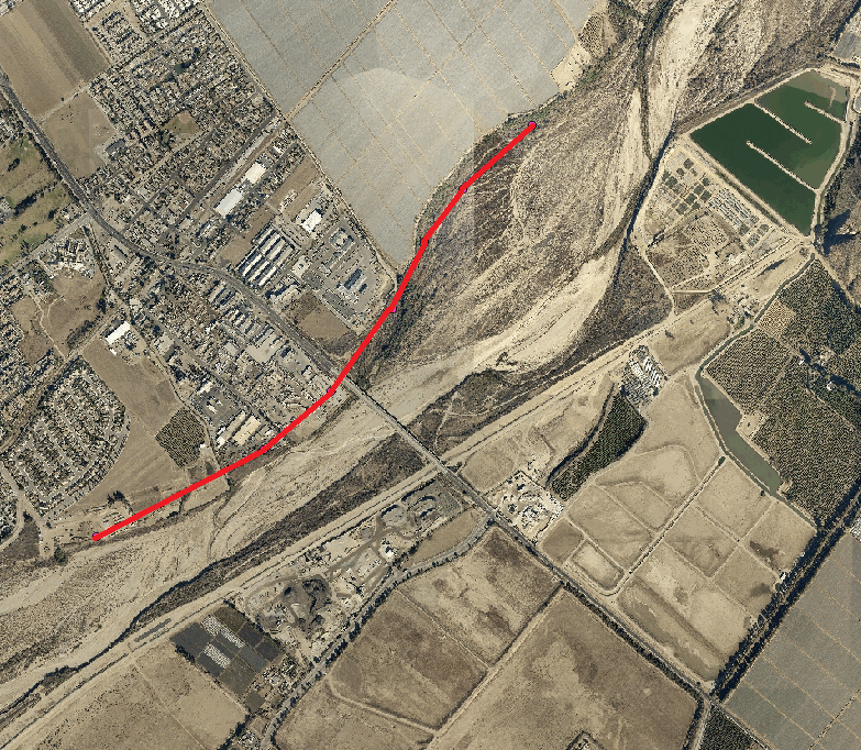
This tutorial illustrates how to incorporate a levee to an existing RiverFlow2D project using the Weirs Component in the QGIS interface. The problem consists in modeling a lateral weir along the right margin of a river, as can be seen in the following figure:

The procedure to incorporate the weir in a RiverFlow2D simulation involves the following steps:

1. Open an existing RiverFlow2D project.

2. Add the Weirs layer.

3. Draw the weir polylines.

4. Input the weir parameters or attributes.

5. Export the files to RiverFlow2D.

6. Run the RiverFlow2D model.

7. Review the output files.

The files required to follow this tutorial can be extracted from the 'ExampleProjects' zip file under the 'WeirTutorial' folder. This zip file is downloaded separately from your installation materials.

Open an existing project

1. Open QGIS.

2. On the Project menu click Open... and browse to select the existing project: .

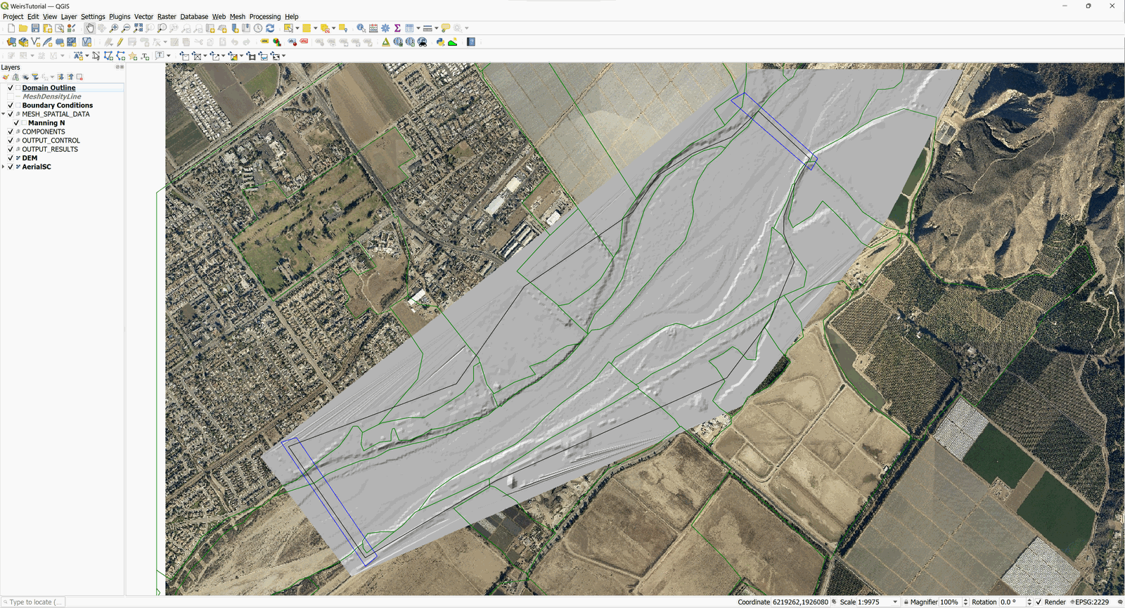
   This project contains the following layers: Domain Outline, Digital Elevation Model (DEM) of the river bed in raster format, aerial photography, polygon with the Manning coefficient and the polygons with the boundary conditions where the flow entrance is in the upper left corner and exit in the lower left corner. The boundary conditions are a hydrograph with a peak discharge of 220,000 \(ft^3/s\), and outflow condition is set to uniform flow. When you open the project you will have a project image loaded in QGIS as shown in Figure 4.2:

Create a Weirs layer and the weir polyline

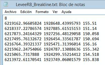
The weir location can be drawn on the Weirs layer or it can be imported from an existing file. In this tutorial, the polyline that indicates the location of the weir will be imported from a text file. The structure of the file should be as follows:

• The first line must indicate the number n of nodes that contains the polyline.

• The n successive lines will contain three columns with the X, Y coordinates.

• The elevation of the weir crest separated by space as shown in Figure 4.3:

Adding the Weirs layer involves the following steps:

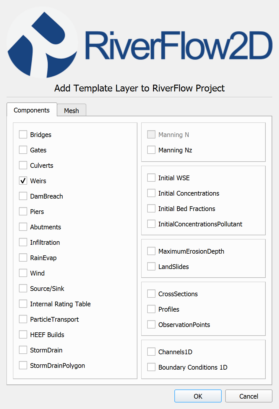
1. Create Weirs layer: for this click on the New Template Layer button in the RiverFlow2D toolbar

   

2. Activate the checkbox Weirs, as shown in the Figure below:

   

3. Edit the Weirs layer: In the layer panel, select the Weirs layer and in the digitization toolbar click on the Toggle Editing button

   

   A pencil icon will appear in the Weirs layer indicating that the layer is in edit mode:

   

4. Draw the line representing the weir: Using the Add Feature tool from the digitization toolbar

   

   Draw a line anywhere in the map area (just mark two vertices or nodes. This line will then be replaced by the coordinates of the file to be imported).

5. Right-click to finish the layout and a dialog window will appear to input the weir parameters.

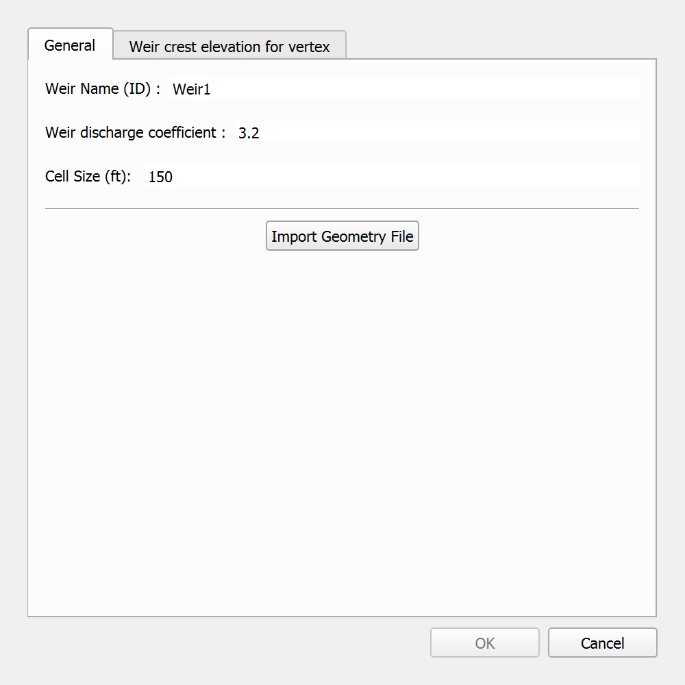
6. Input the weir parameters: The window to input the weir attributes contains two tabs. In the first one there are the fields of the general parameters, within which has:

   • Weir Name (ID): Weir1

   • Weir discharge coefficient: 3.2

   • Weir crest elevation for all the weir: since a file will be imported this field will be left empty.

   • Size Element: 150

   • Import Geometry File: Click the [...] button and point to the file LeveeRB_Breakline.txt which is found in the tutorials folder.

   The weir parameters window should look like the image shown below:

   

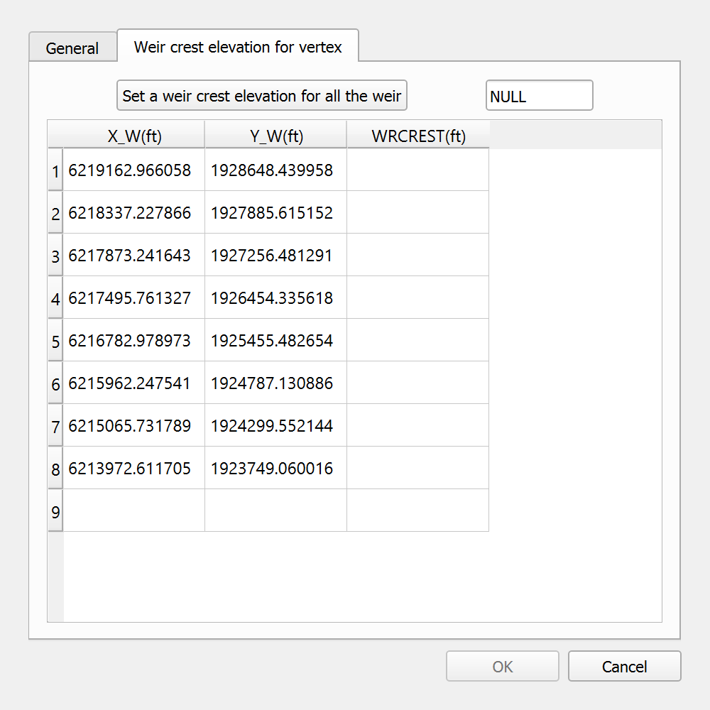
   In the second tab 'Weir crest elevation for vertex' the data contained in the file LeveeRB_Breakline.txt is displayed, as shown in the following Figure:

   

7. Then click on the [OK] button.

8. Save the changes in the layer using the Save button of the digitization toolbar

   

9. Disable the editing mode of the layer with the Toggle Editing button

   

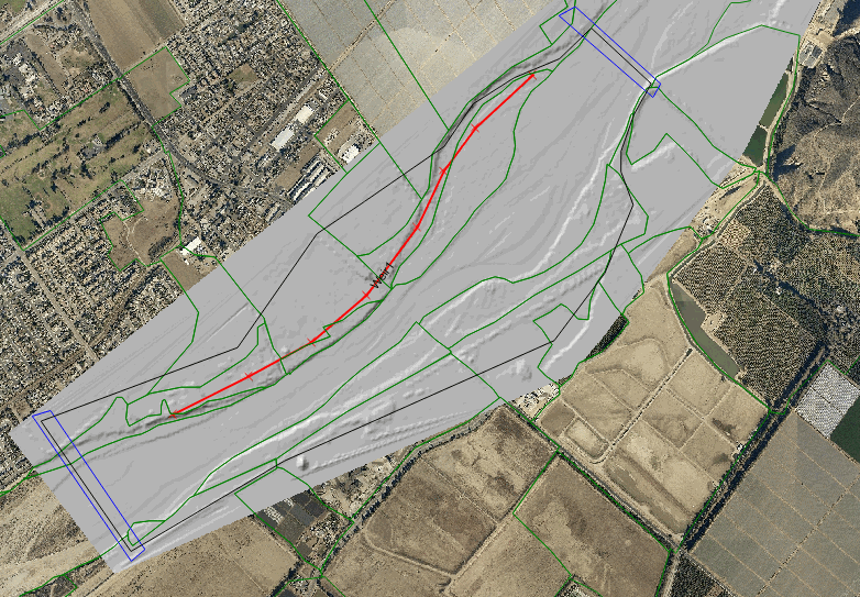
   and we will have on screen an image similar to the one shown below where you can see the layout of the weir:

   

Generate the mesh

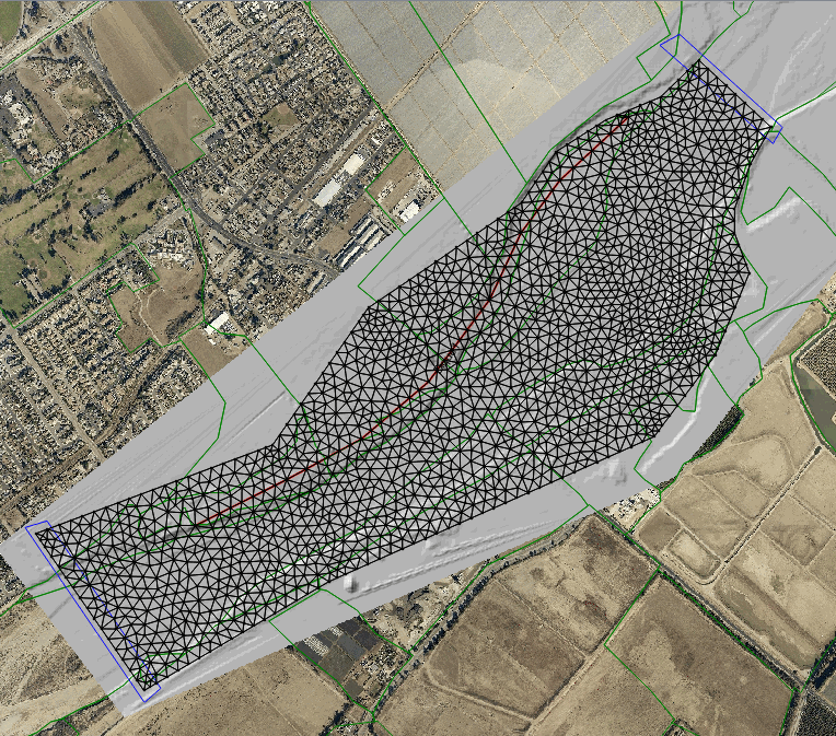
The mesh is generated with the Generate TriMesh plugin.

result should look similar to the image on Figure 4.8.

Exporting files to RiverFlow2D

Now that you have generated the mesh and you have the other layers ready with the necessary data, you should export the files in the format required by RiverFlow2D.

1. Click the *Export to RiverFlow2D * button.

   

2. When running the plugin a window is displayed, here we must select the raster layer that contains the Digital Elevation Model (DEM) and the name of the project to be exported.

   Once the plugin is executed, a window will be shown (Figure 4.9), as it should be for our example.

3. After inputting the data, click the OK button and wait for the export process to finish.

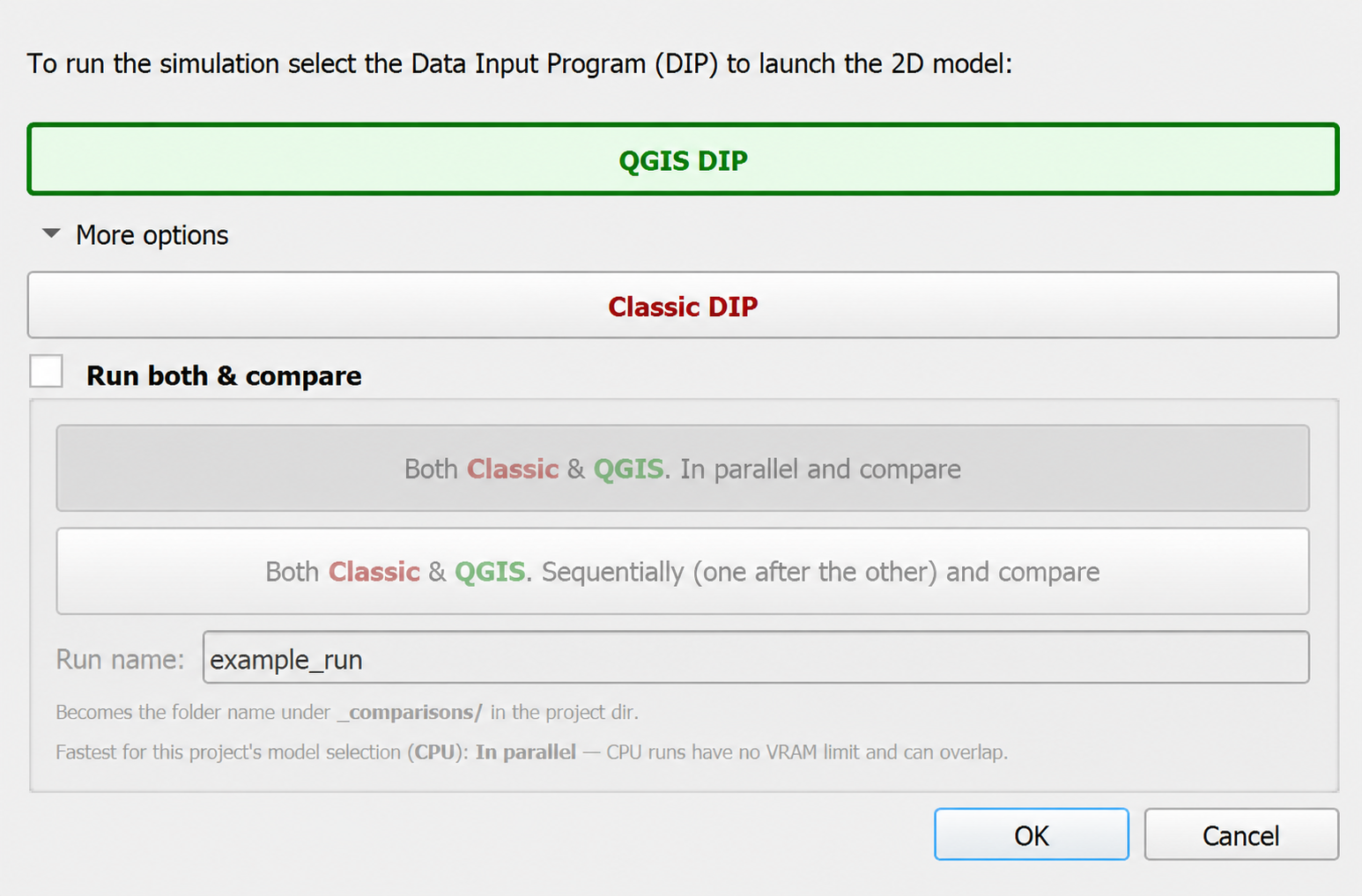
   In Hydronia2DMS version 10 and later, the Open DIP dialog appears after export. QGIS DIP is selected by default; click OK to open it inside QGIS. To use the historical standalone option, expand More options, select Classic DIP, and then click OK.

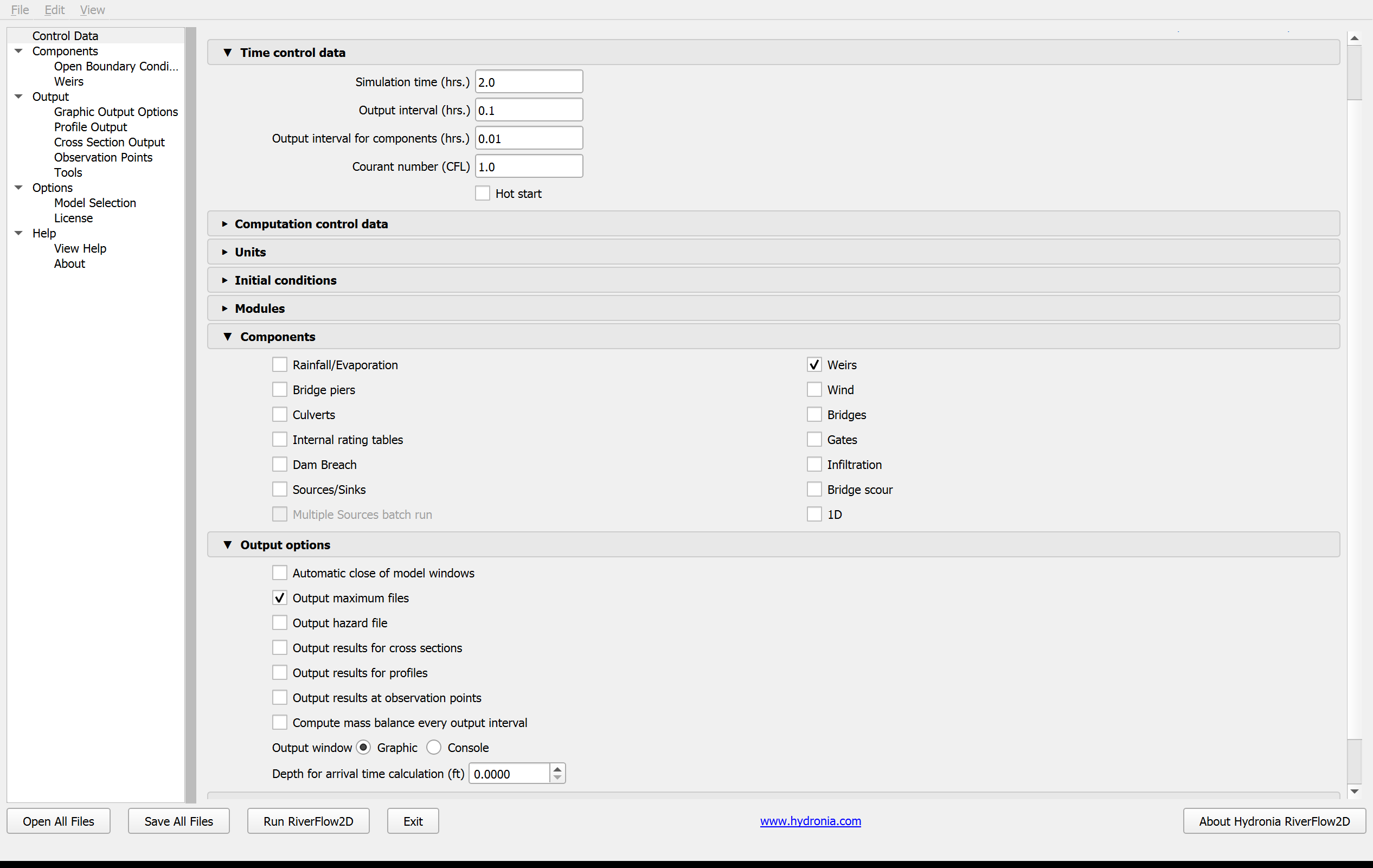
4. Open the selected DIP. QGIS DIP displays the model controls inside QGIS:

   

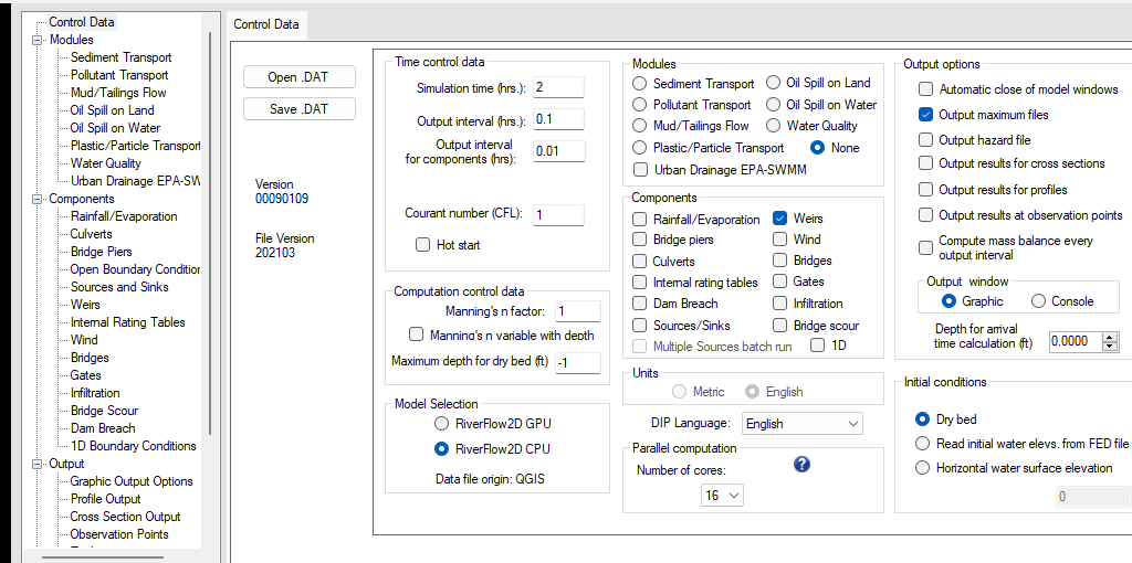
   The following Classic DIP Control Data panel is retained as a legacy values reference:

   

Running the model

Make sure that the Weirs component is selected in the Control Data panel. The controls are equivalent in QGIS DIP and Classic DIP, although their appearance differs.

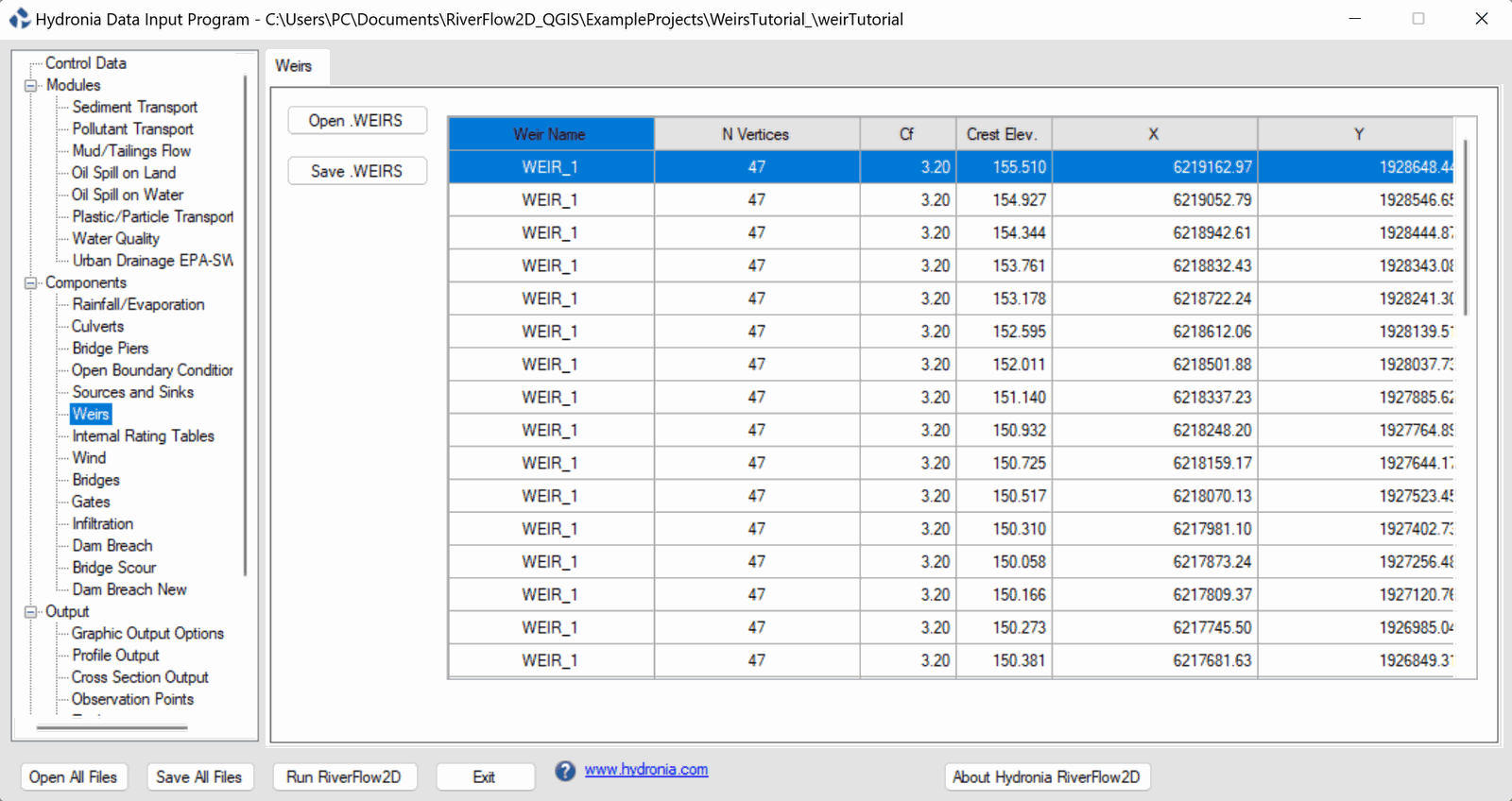
1. In the list of components, select 'Weirs' and the panel of the Weirs component will appear. In this window the contents of the '.WEIRS' file content as prepared by RiverFlow2D will be displayed (Figure 4.11).

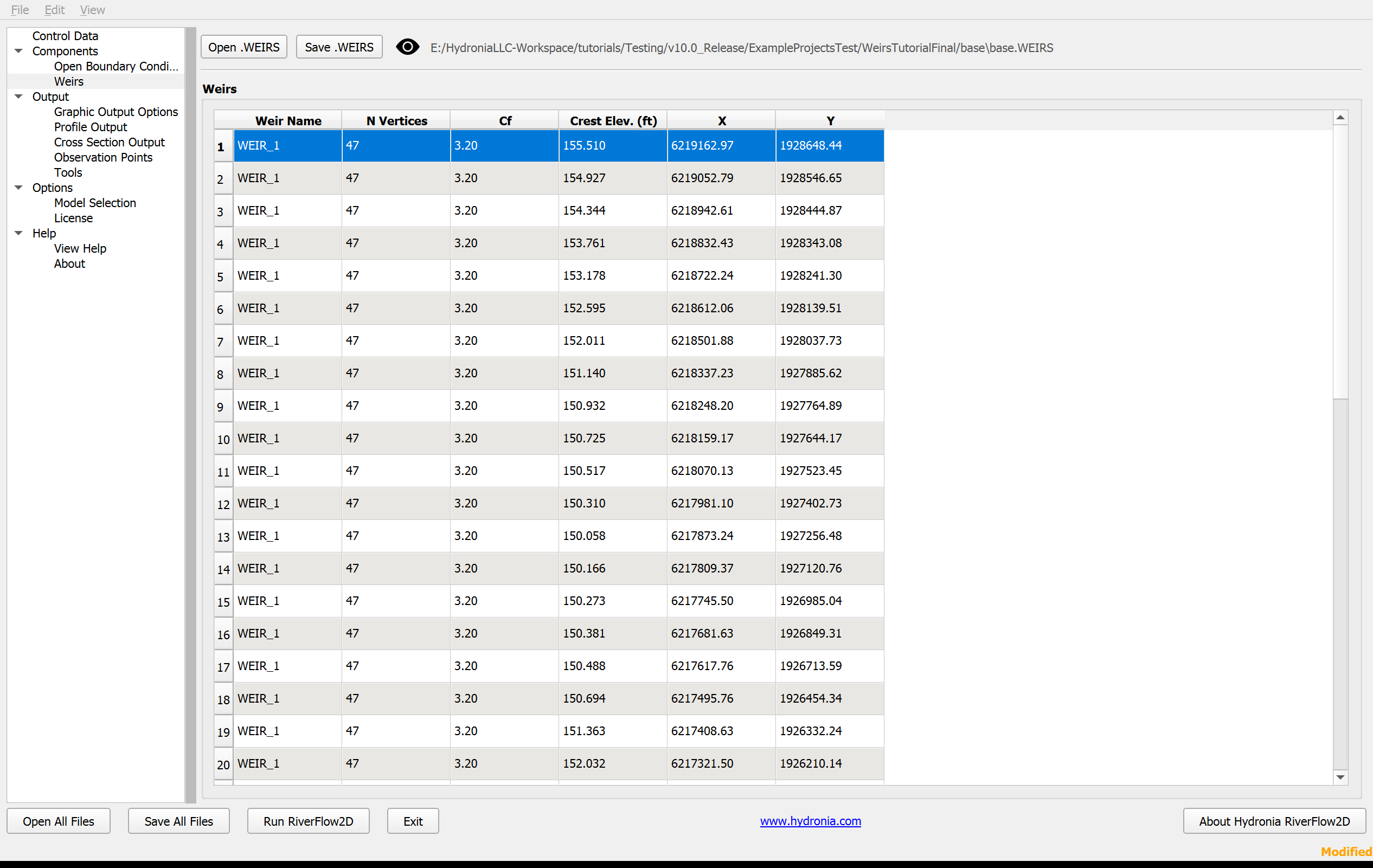
   The following Classic DIP panel is retained as a legacy values reference:

   

2. Leave all other parameters at their default values.

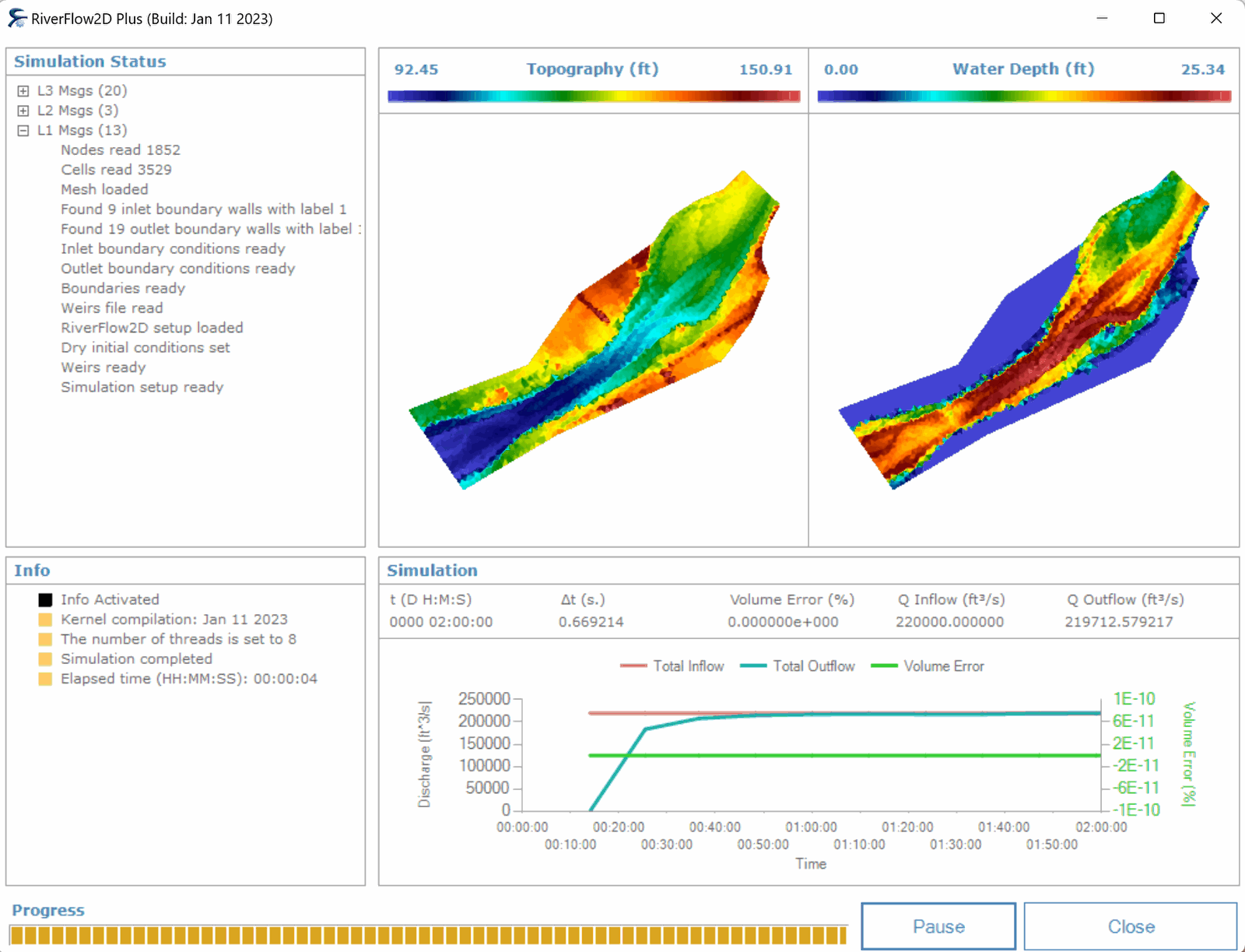
3. Click the Run RiverFlow2D button. The model status window reports the simulation time, volume conservation error, and total input and output discharge as execution progresses. When the run finishes, confirm that the completion status is shown before closing the window (Figure 4.12).

Review the output files

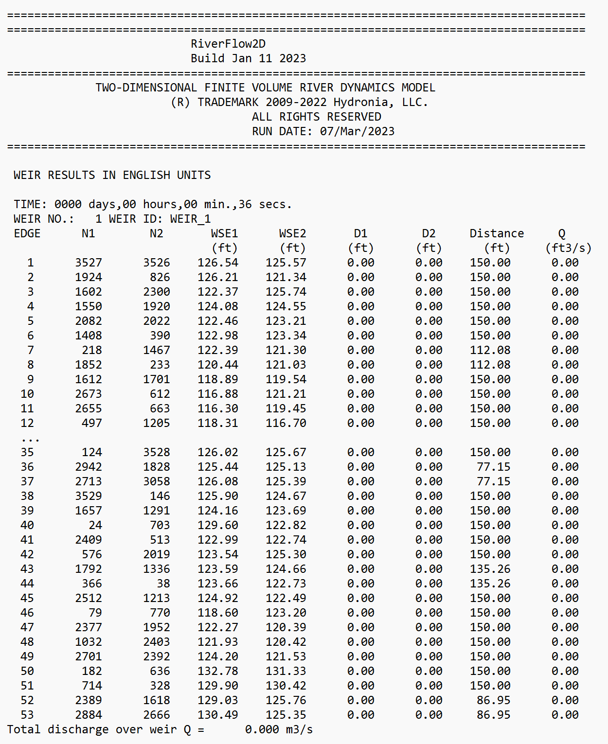
RiverFlow2D creates an output file with the name of the project and extension '.WEIRI' for metric units and '.WEIRE' for English units. The files report results for each weir and for each output interval. Output includes the following information:

• EDGE: The segments into which the weir is divided and is given by the length of the cells in contact with the weir.

• N1 y N2: The numbers that identify the cells that share the EDGE segment in the weir.

• WSE1 y WSE2: The elevations of the water surface in the cells indicated by N1 and N2.

• D1 y D2: The depths of the flow in the cells indicated by N1 and N2.

• Distance: The length of the EDGE segment.

• Q: The discharge that passes through the EDGE segment.

The '.WEIRE' file contains the following:

This concludes the Simulating Levees using Weirs Tutorial.