Simulating Oil Pipeline Breaks

This tutorial will explain how to use the OilFlow2D model to simulate oil spills from a pipeline utilizing the Oil Pipeline Module. The steps to accomplish this are as follows:

1. Starting QGIS and Creating a new OilFlow2D project.

2. Adding the required layers.

3. Create the Pipeline by adding the Oilpipeline layer.

4. Running the Oil Pipeline Break Module within the OilFlow2D plugin.

5. Generating the triangular mesh and exporting the data files to the OilFlow2D model.

6. Configuring parameters in the Hydronia Data Input Program.

7. Creating maps of all sources from results data.

Tutorial data

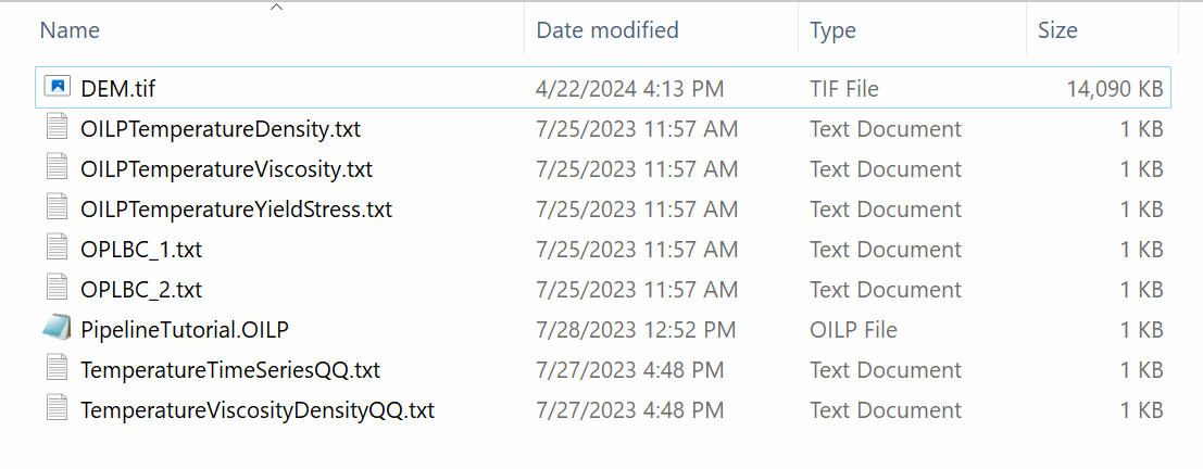
The files required to follow this tutorial can be extracted from the 'ExampleProjects' zip file under the 'SimulatingPipelines' folder. This zip file is downloaded separately from your installation materials. The folder contains the files shown:

Starting QGIS and Creating a new OilFlow2D project

1. To create a new OilFlow2D project, open QGIS and then click on the New OilFlow2D Project button in the toolbar. A dialog window appears where you select the optional component layers, the Coordinate Reference System (CRS), the initial scenario name, and the project directory. For this example, select none in Layers, choose EPSG:2202, keep Name initial scenario set to base, and use SimulatingPipelines as the Project Directory.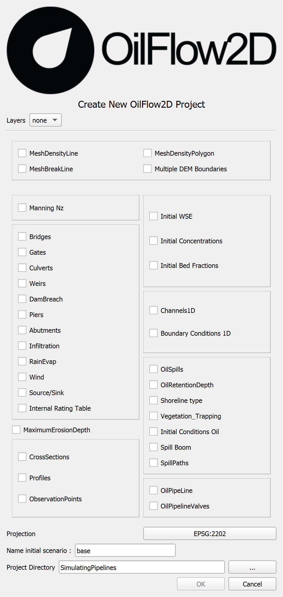

   

   Copy all of the files from the SimulatingPipelines tutorial folder into the new scenario folder created. In this example it would be copied into \SimulatingPipelines\base.

2. Save the QGIS project by clicking on the Save Project icon in the toolbar.

3. Make sure to save the QGIS project above the scenario folder. In this example it would be saved under \SimulatingPipelines\.

Setting up the required layers

The Digital Elevation Model (DEM) or Digital Surface Model (DSM) needs to be added to the project, then the Domain Outline, Manning N will need to be drawn and given input values.

1. In this tutorial we will load a DSM clicking the Add Raster Layer button . You may also use the QGIS shortcut Control+Shift+R.

   The DSM file DEM.tif is located in the extracted SimulatingPipelines tutorial folder.

2. Drag the newly added DSM layer to the bottom of the list in the Layers panel:

   

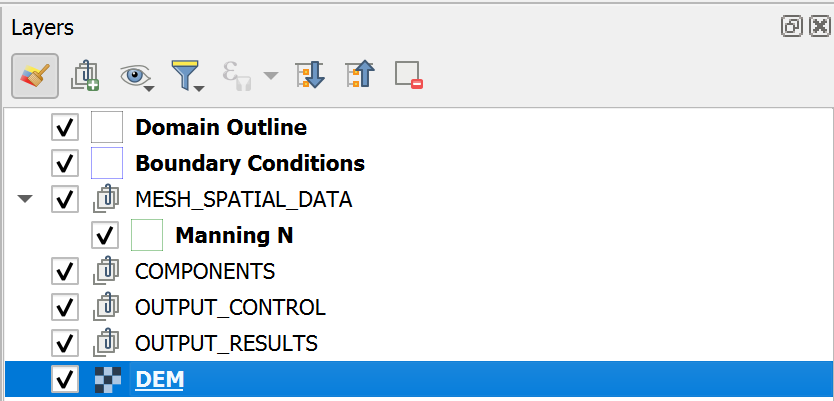
   Right-clicking on the label of the new raster layer and selecting Properties, in the Symbology panel you can change the Render type for a more informative palette such as Hillshade for instance.

3. Right-click the DEM layer and select Zoom to layer(s).

   This is what you should have on your screen so far:

   

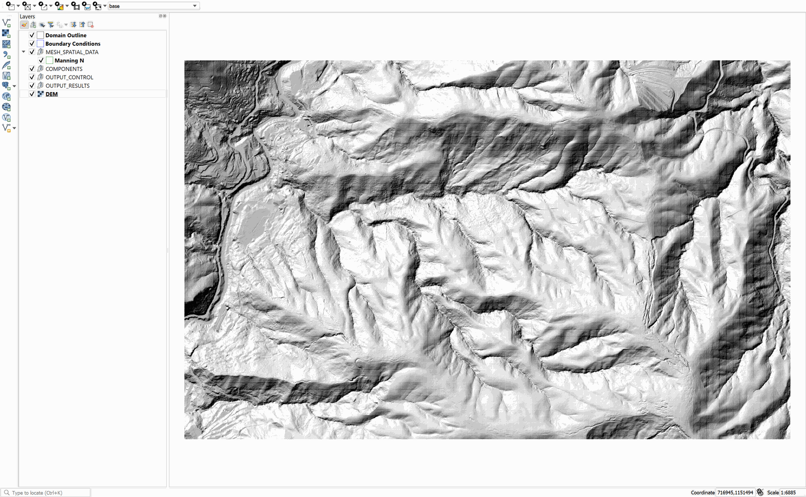
4. The limits of the modeling area are defined using a polygon on the Domain Outline layer. To create it do as follows: Select the Domain Outline layer in the Layers panel and click on Toggle Editing icon in the toolbar section.

5. Click the Add Polygon Feature tool . Proceed to delineate the outline of the polygon by clicking the vertices with the left mouse button as shown: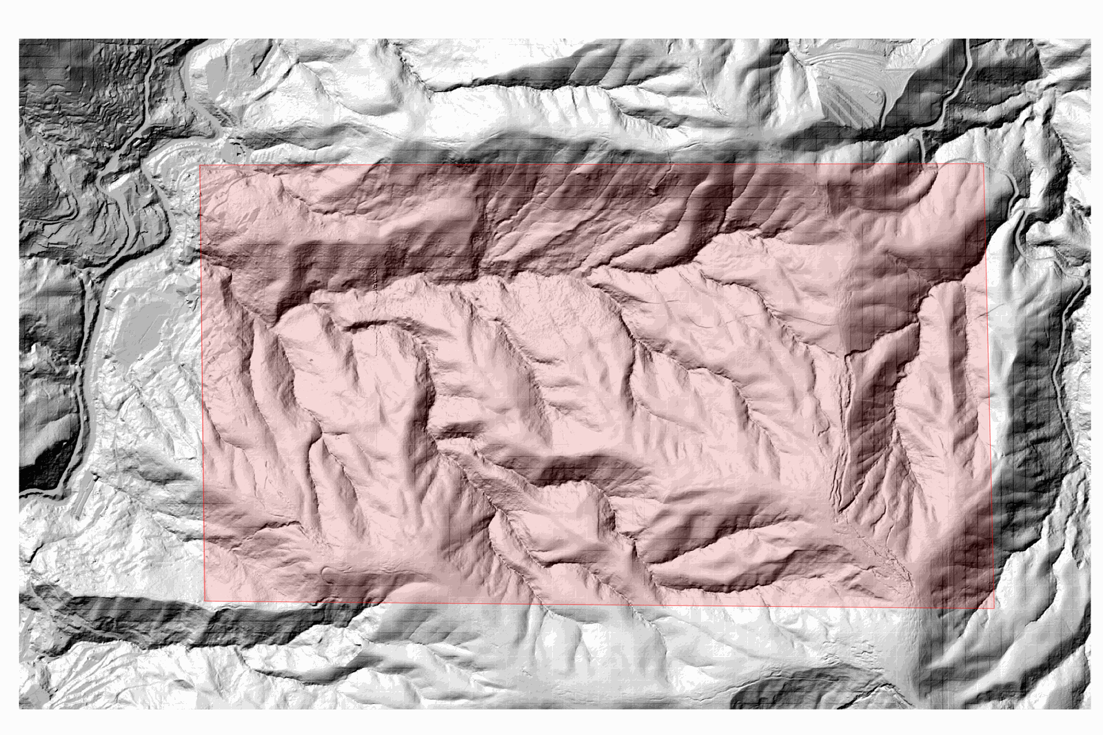

   

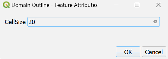
6. Right-click to close the polygon. A dialog will appear asking for the Cellsize value for our mesh. Input 20 as our value.

   

7. Click the Save icon and then click the Toggle Editing icon to deactivate editing mode.

8. Now that we have created the Domain Outline, deactivate the Boundary Conditions layer by unchecking the box on the left side, as it will not be used for this exercise.

9. Select the Manning N by clicking on the layer located under the MESH_SPATIAL_DATA group.

10. Click on Toggle Editing icon in the toolbar section.

11. Click the Add Polygon Feature tool . Proceed to delineate the outline of the polygon by clicking the vertices with the left mouse button, keeping the polygon outside of the Domain Outline polygon as shown: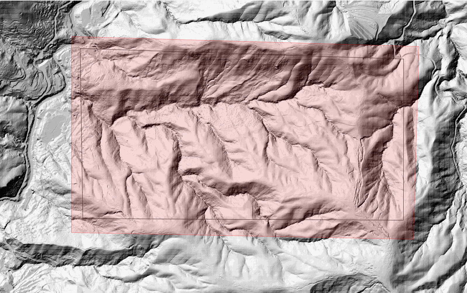

    

12. Right-click to close the polygon. A dialog window will appear to input the Manning N coefficient. Enter the value 0.03.

13. Deactivate the Boundary Conditions layer in the Layers panel by clicking the checkbox on the left side. It will not be used in this tutorial.

14. Click the Save icon and then click the Toggle Editing icon to deactivate editing mode.

15. Save the QGIS project by clicking on the Save Project icon in the toolbar.

Create the Pipeline by adding the Oilpipeline layer

A polyline will be used to delineate the location and length of the pipeline for this tutorial. First, a the Oilpipeline layer must be created:

1. Click on the OilFlow2D Tools dropdown menu and select New Template Layer.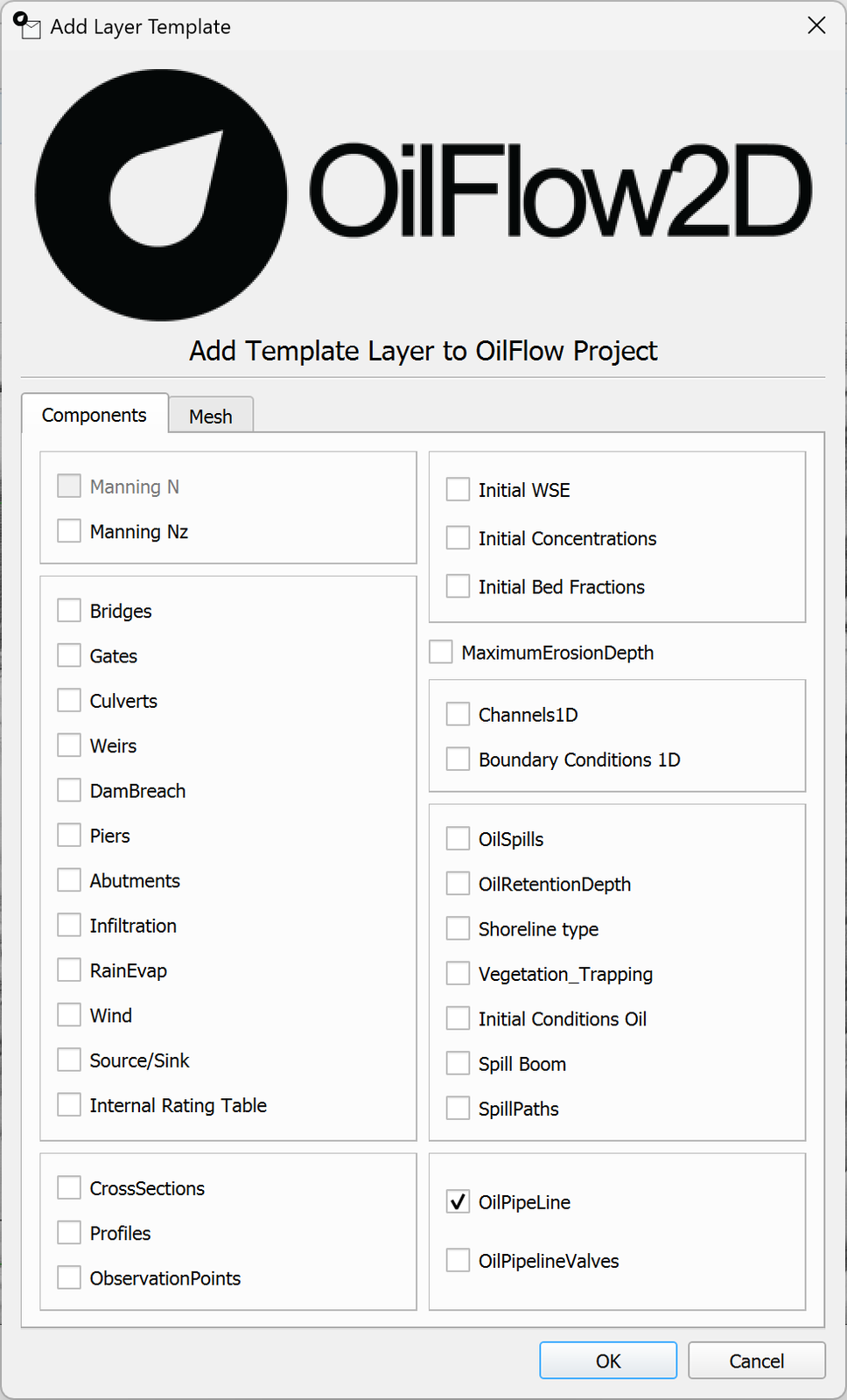

   

2. Click [OK] in the Add Layer Template window.

3. Select the OilPipeLine layer in the Layers panel and click the Toggle Editing icon in the toolbar section.

4. Click the Add Line Feature button and then start to draw the pipeline on the map by left-clicking to create the vertices.

5. Right-click to end drawing the pipeline. A dialog window will appear requesting to add additional data about the pipeline. Keep default values and make the pipe diameter 3 meters as shown:

   

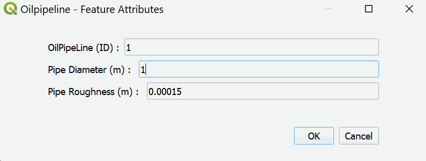
   The finished pipeline should look similar to the following:

   

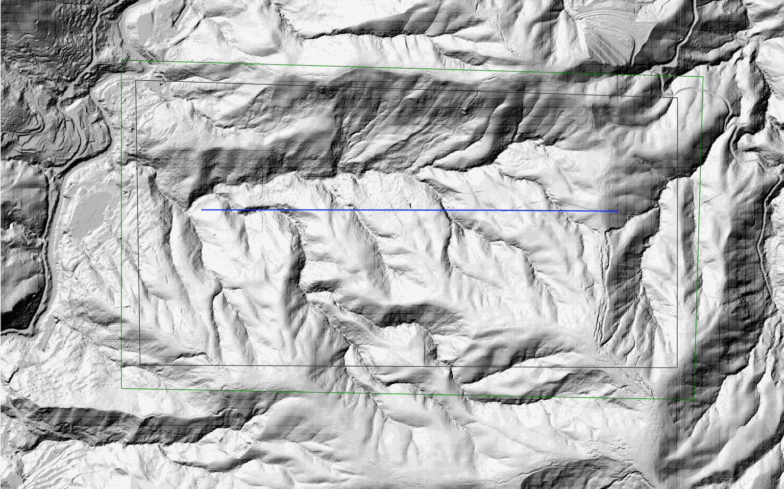
6. Save the QGIS project by clicking on the Save Project icon in the toolbar.

Running the Oil Pipeline Module within the OilFlow2D plugin

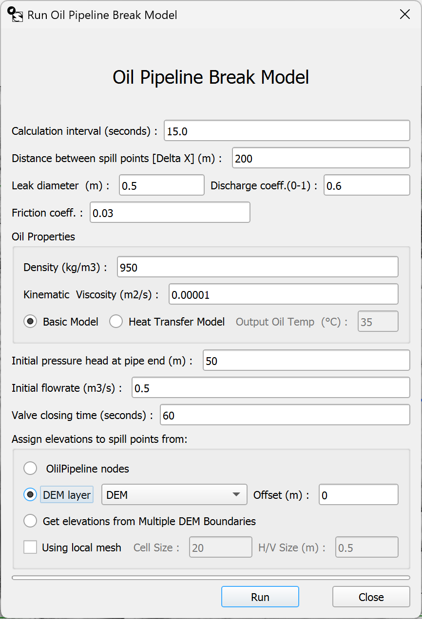
The Oil Pipeline Break Model tool will be used in this tutorial to create the sources of the spill along the length of the pipeline. It requires us to specify the length between each break, the total inflow rate, the oil properties, and will calculate the spill outflow rates for each break based on these parameters.

1. Click on the OilFlow2D Tools dropdown menu and select Run Oil Pipeline Break Model.

2. Enter the data as shown in the following figure:

   

3. Click [Run]. The plugin will generate a new Sources layer, populate it with the spill points and they will appear along the pipeline in the map area:

   

4. Save your QGIS project by clicking on the Save Project icon in the toolbar.

Generating the triangular mesh and exporting to the OilFlow2D model

1. Create the mesh with a cell size of 20 meters by clicking on the Generate Trimesh button.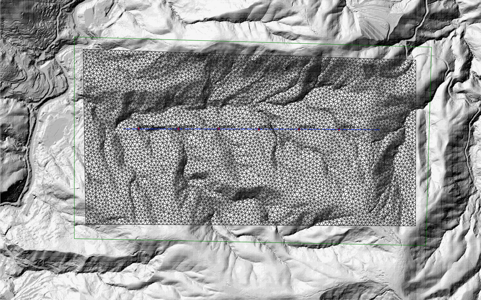

   

2. Save your QGIS project by clicking on the Save Project icon in the toolbar.

3. Click on the Export files for OilFlow2D dropdown and select Export Hydrodynamic OilFlow2D.

4. Leave all default values and click [OK] to export.

   After export completes, version 10 and later users see the Open DIP dialog. QGIS DIP is selected by default; click OK to open it inside QGIS. To use the historical standalone option, expand More options, select Classic DIP, and then click OK.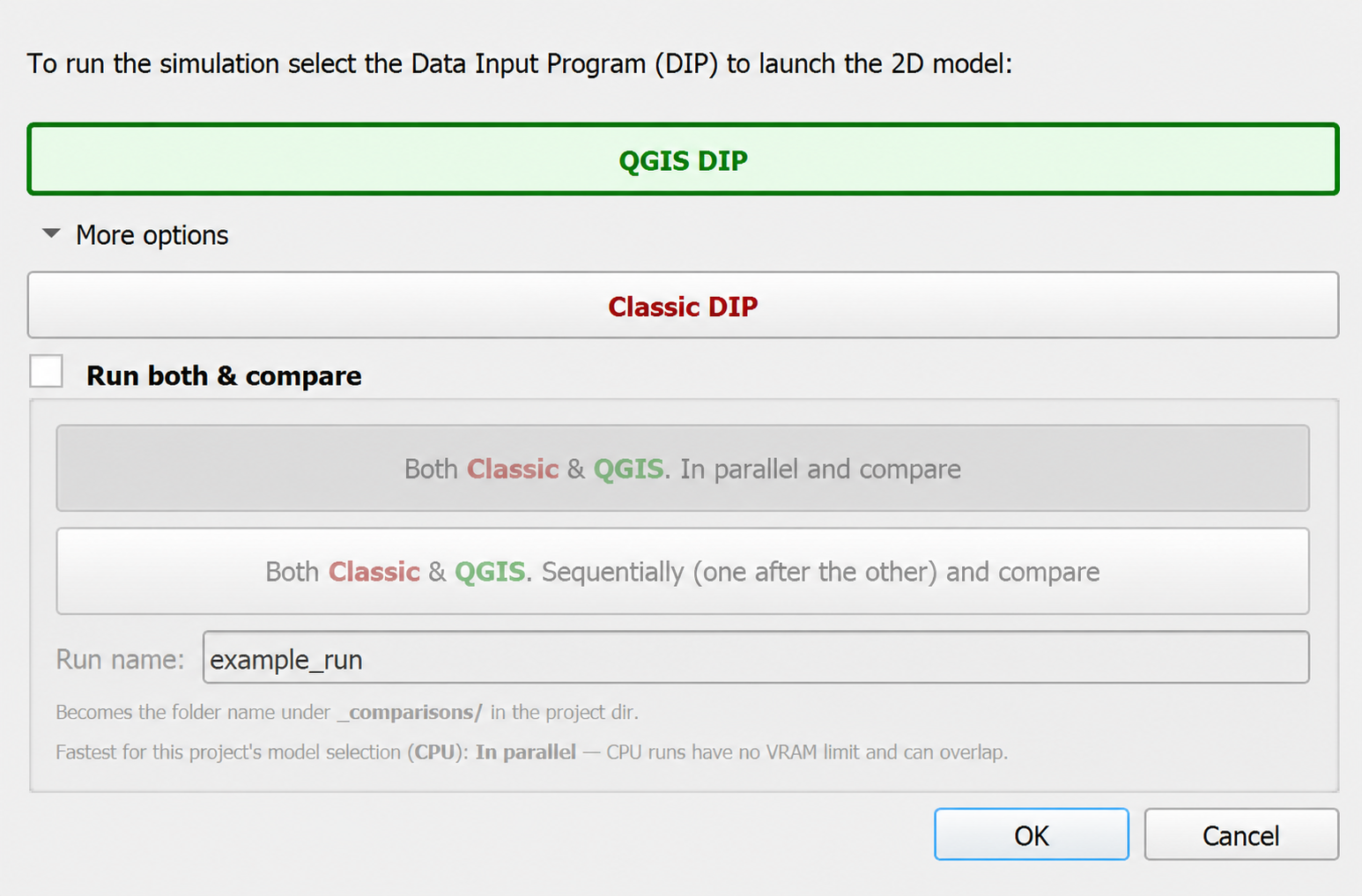

   With QGIS DIP selected, the current interface is shown below: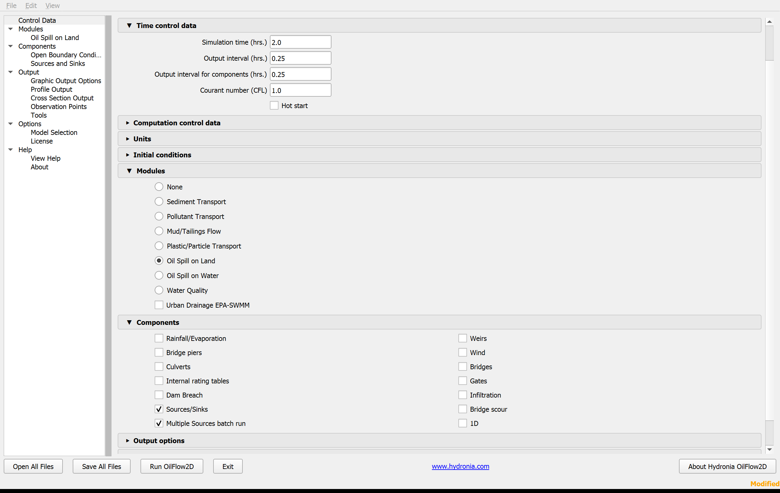

   

   QGIS DIP and Classic DIP use the same project settings, but their interfaces look different. Older standalone or non-maintenance versions may open Classic DIP automatically. The project-specific Classic DIP settings and Run steps below are retained.

Configuring parameters in the Hydronia Data Input Program

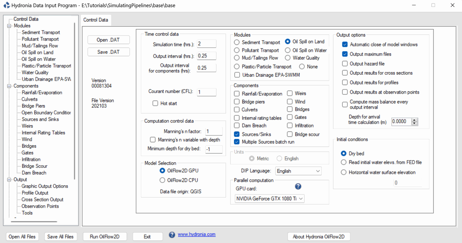
The tutorial will simulate pipeline breaks at each of the spill points for 2 hours with 15 minute intervals. Please do the following:

1. Configure the Control Data parameters with the parameters in the figure below:

   The following Classic DIP Control Data panel is retained as a legacy values reference:

   

2. Click on the Oil Spill on Land module in the left pane of the DIP.

3. Click on the [Open .OILP] button.

4. Browse to the 'SimulatingPipelines' folder and select the 'PipelineTutorial.OILP' then click [OPEN].

   The Oil Spill on Land window should look like the figure below:

   

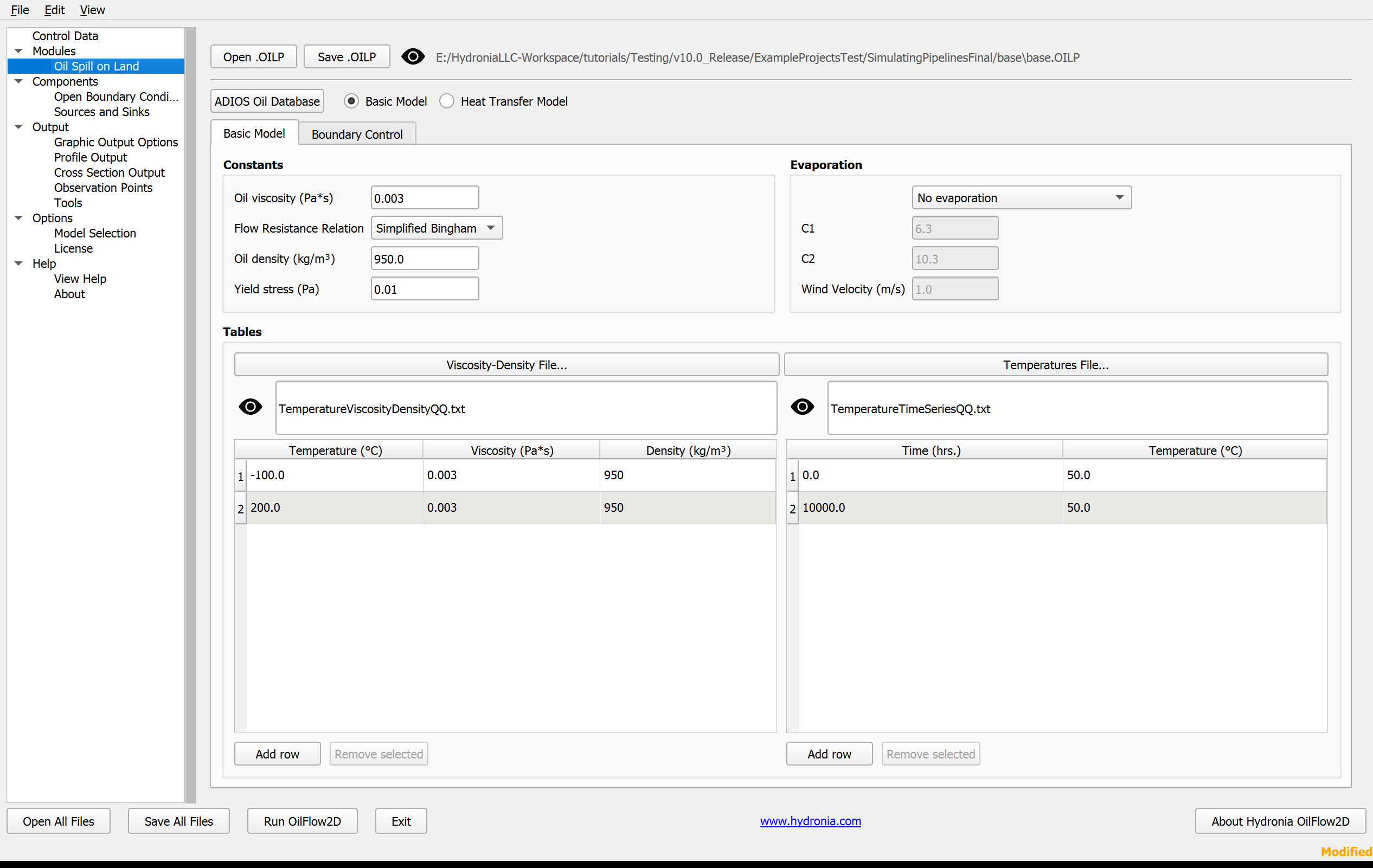
   The following Classic DIP Oil Spill on Land panel is retained as a legacy values reference:

   

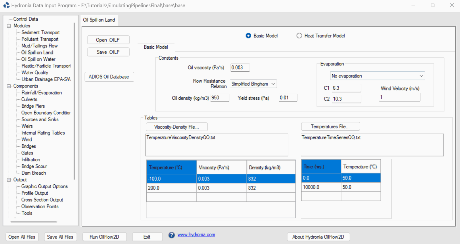
5. Click the [Save .OILP] button. Keep the default name (The name of the scenario in your case). Click [Save].

6. Return to the Control Data pane and Click [Run OilFlow2D].

7. When asked to save the DAT file, Click [Yes] and click [Save], making sure it is in the default project directory with the name provided.

   Multiple model windows will appear and close automatically during the simulation process, they will look like the following figure:

   

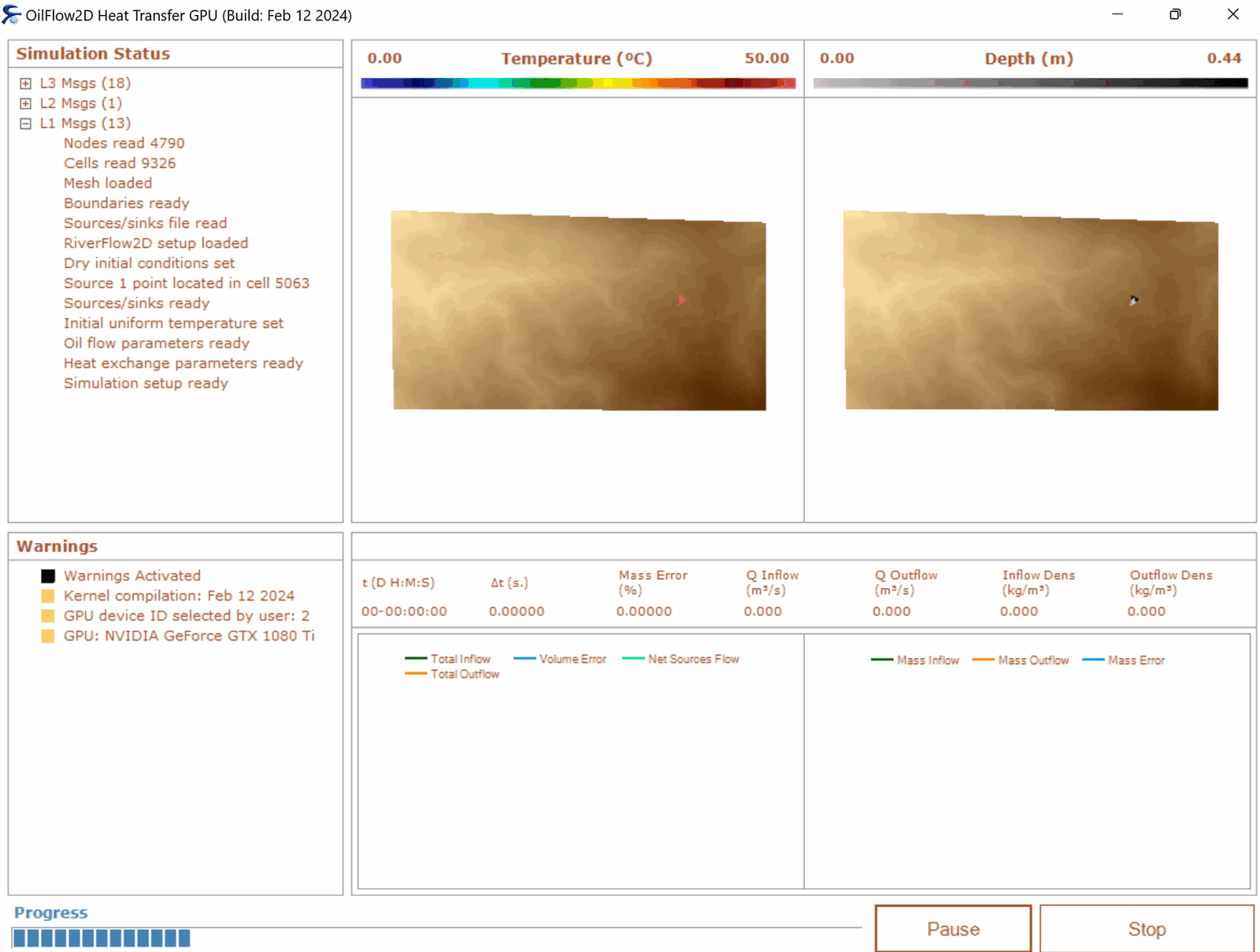
   When this process ends, the windows will all be closed automatically. The model has finished simulating all sources.

Creating maps of all sources from results data

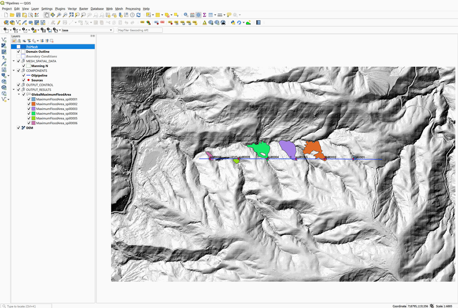
The OilFlow2D plugin for QGIS can create a single layer with the results of the multiple pipeline breaks. In this example a map of the combined spill affected area will be created. This can be performed with the following steps:

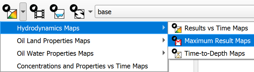
1. In the OilFlow2D Maps dropdown button in the OilFlow2D toolbar, click on Hydrodynamics Maps and then Maximum Result Maps.

2. Click the [. . .] button to specify the Maximum Value File. A dialog will appear.

   

3. Browse into the newly created results folder, named 'spill0001'. Select the file with your project name _cells_max.textout. In this example the file is named 'Pipelines_cells_max.textout'. Click [Open].

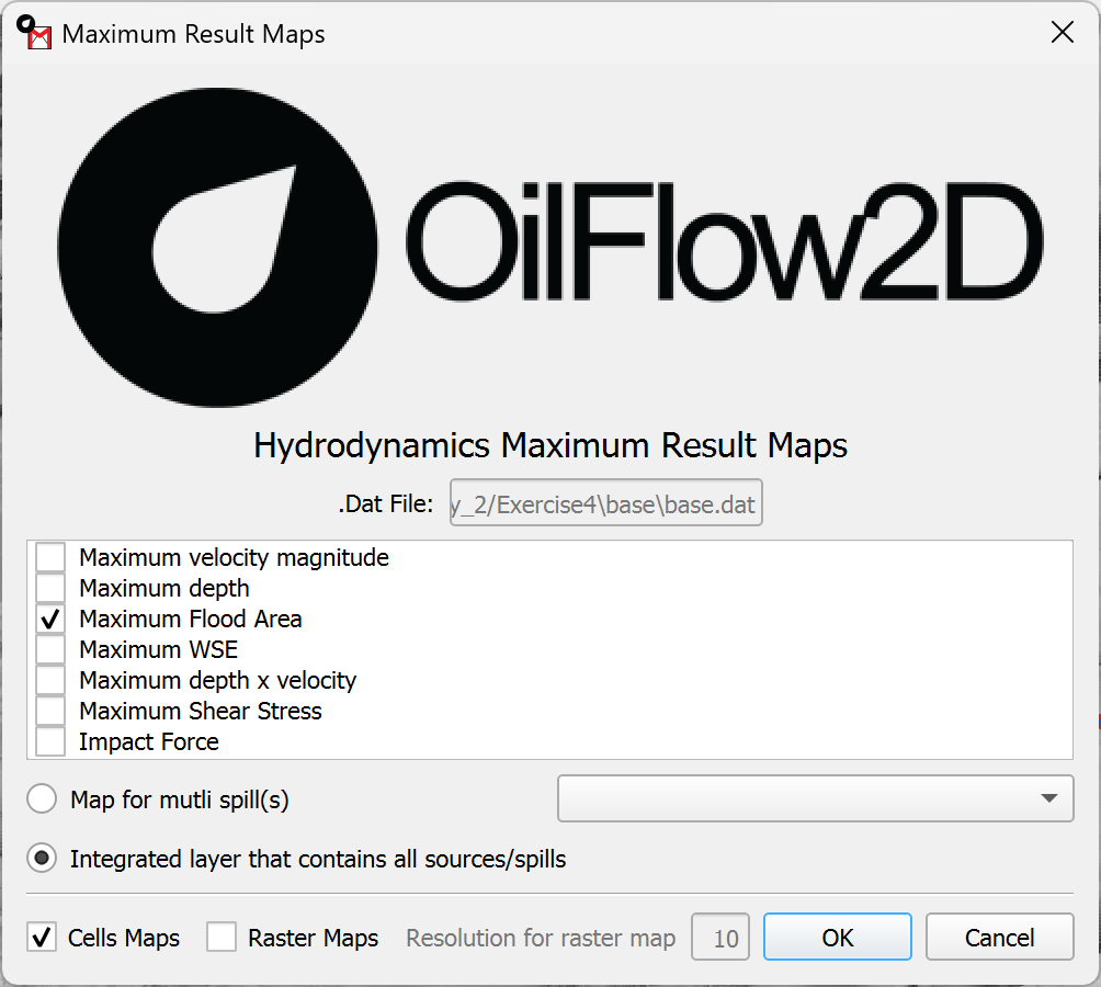
4. A list will appear in the Maximum Result Maps window. Click the checkbox for Maximum Spill Area, and select the radio button for Integrated layer that contains all sources/spills, then click [OK].

   

   After classifying the spill-area polygons by the layer attribute that corresponds to the spill point, the final result should look like the following:

   

   This concludes the Simulating Oil Pipeline Tutorial.