Wind driven circulation

OilFlow2D and OilFlow2D allow defining wind velocity on the water surface to account for the effect of the wind stress on the flow velocities. The conceptual model of a wind driven simulation require a series of non-overlapping polygons that determine the wind velocity data to the model. Only areas covered by polygons will be affected by the wind stress. Each wind velocity polygon should be associated with a file containing a wind velocity time-series file containing the two components of the wind velocity vector for each time. The user will need to generate the wind velocity data file associated with each polygon, and copy them to the project folder, prior to running the model.

This tutorial illustrates how to perform a wind drive simulation using the QGIS interface. The procedure includes the following steps:

1. Create time series data for wind speed.

2. Open an existing OilFlow2D project.

3. Create the template of the wind layer and the wind speed polygons.

4. Generate the mesh.

5. Running the model.

6. Review wind output files.

The files required to follow this tutorial can be extracted from the 'ExampleProjects' zip file under the 'WindTutorial' folder. This zip file is downloaded separately from your installation materials.

Open an existing project

1. Open QGIS

2. On the Project menu click Open... to load the existing project: 'WindTutorial.qgz'.

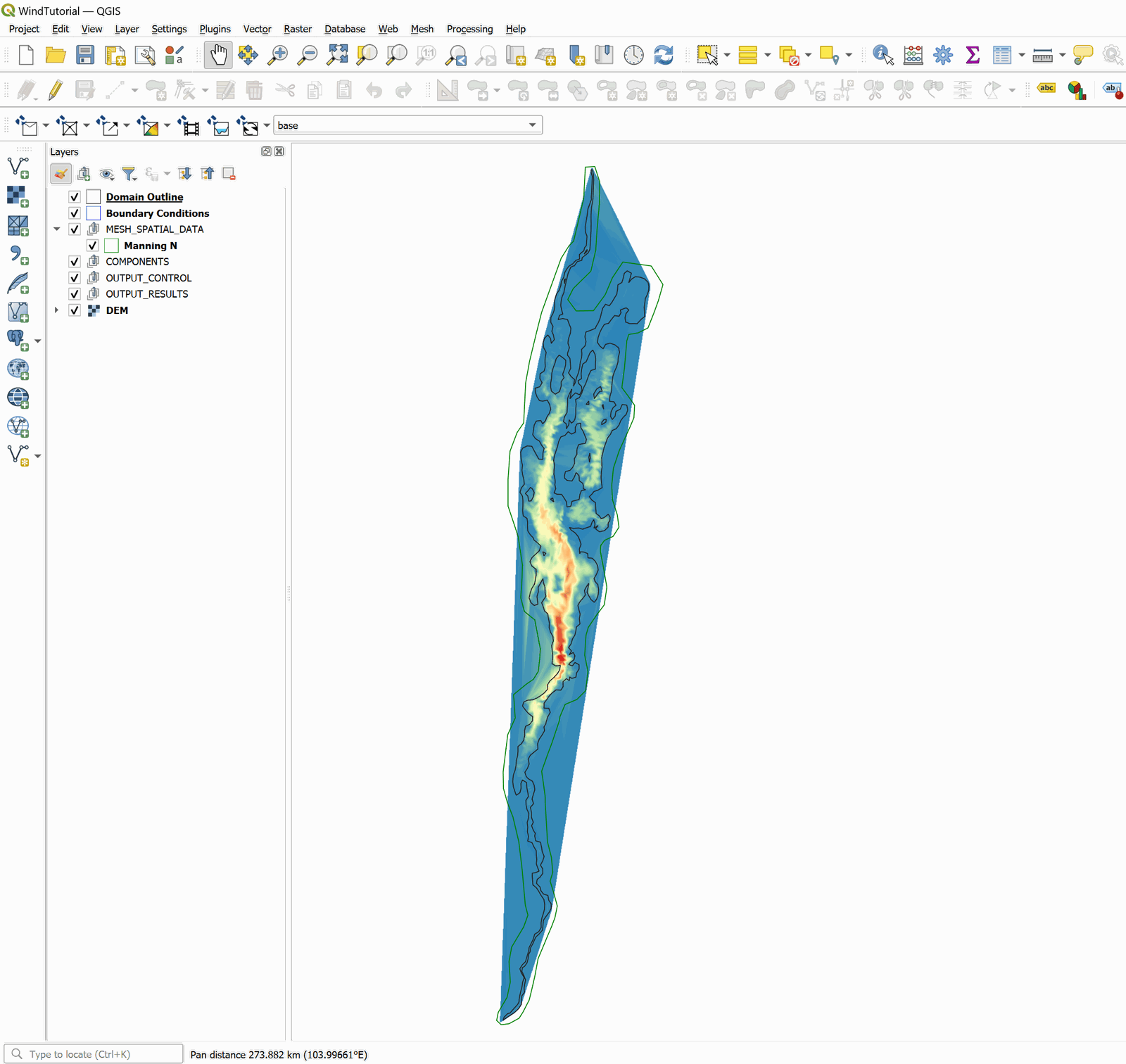
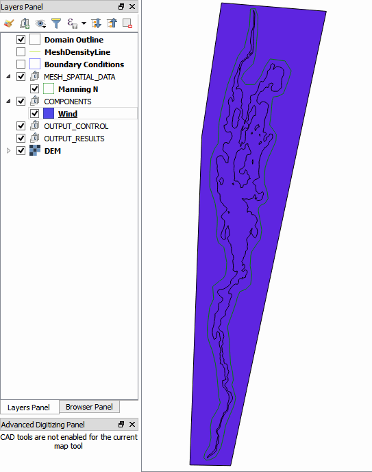
This project contains the layers of the domain contour and the layer of the Digital Elevation Model (DEM) of Lake Champlain in the USA. When the project is opened, a project image will be loaded in QGIS as shown in Figure 15.1.

Wind velocity time-series data file

To run a wind driven simulation you create polygons over which the wind velocity data will be applied. Each polygon will have an associated velocity time series. These files can be created with any text editor such as Notepad or Wordpad. The wind velocity file has the following format:

Line 1: Number of points in the time series of wind velocity

NP

NP lines containing:

TIME Wvx Wvy

where Wvx and Wvy, are the wind velocity components in x and y directions respectively in m/s or ft/s.

The following table is an excerpt of the 'WindVelocDATA.TXT' file that is included in the Data folder for this tutorial:

6544
0        5.97       -2.17
1        5.09        8.83
2        3.84        6.63
3        5.87        4.92
4        0.00        0.00
5       -3.31       -1.90
...
6543     3.84       -6.63

Create the template for the wind layer and the wind speed polygons

To add the template where the polygons are drawn with the wind speed time series data involves the following steps:

1. Create the template for the Winds layer: In the model toolbar click on the New Template Layer command

   

2. The existing WindTutorial.qgz project uses the base scenario and EPSG:6623. In the Add Template Layer to OilFlow Project window, activate the Wind checkbox, as shown in the Figure below: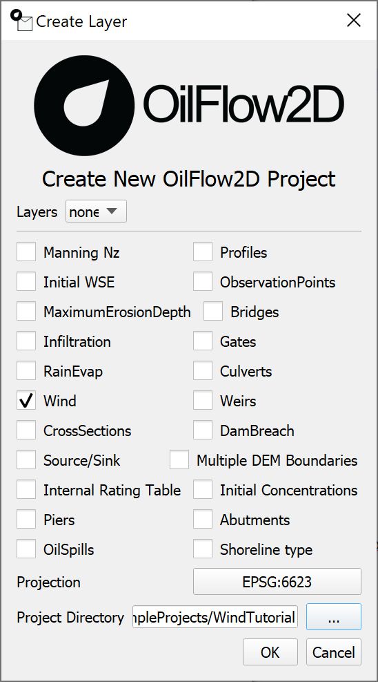

   

3. Edit the Wind layer: In the layers panel, we select the Wind layer and in the digitization toolbar we click on the Toggle Editing tool . A pencil icon will appear in the Wind layer, indicating that the layer is in edit mode:

   

4. Draw the polygon that demarcates the Wind area: Using the Add Feature tool from the digitization toolbar .

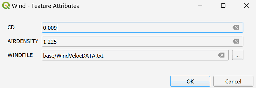
   Draw the polygon that defines the wind area. In this case, the tracing of the polygon must be done in such a way that it covers all the cells of the mesh. Once you finish drawing the polygon a window to input the polygon parameters is immediately opens, which are three:

   • Wind stress coefficient CD: 0.009,

   • Air density: 1.225, and

   • Wind speed time series File: 'WindVelocDATA.txt'.

   The parameter window should be as shown below:

   

5. After input the values, click OK and accept the changes. There should be an image similar to the one shown in the following figure:

   

Generate the mesh

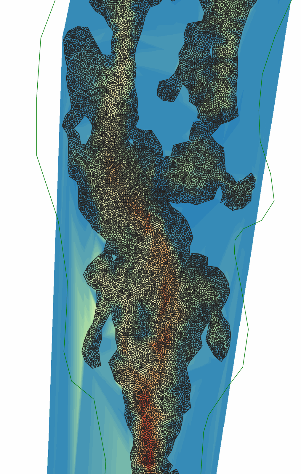
Then the mesh is generated with the Generate TriMesh button

The results obtained as shown in Figure 15.5 (mesh of around 17,500 cells).

Exporting files

After generating the mesh and preparing the other layers, export the files in the format required by OilFlow2D.

1. Uncheck the Boundary Conditions layer.

2. Activate the DEM layer.

3. Use the Zoom Full button to center the image if required.

4. Open Plugins > OilFlow2D MS > Export OilFlow2D and click the exact visible action Export Hydrodinamic OilFlow2D.

   

5. In the OilFlow2D export dialog, keep the Scenario Name value at base and choose DEM in the DEM (Single Raster) field. The dialog labels the operation Export Files to OilFlow2D.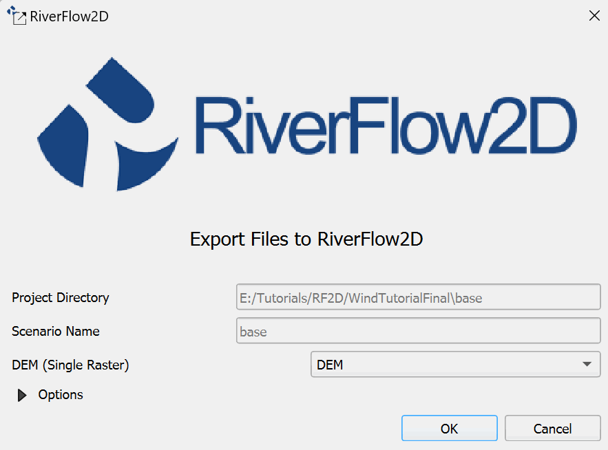

   

6. Click OK after checking the values.

   After export completes, version 10 and later users see the Open DIP dialog. QGIS DIP is selected by default; click OK to open it inside QGIS. To use the historical standalone option, expand More options, select Classic DIP, and then click OK.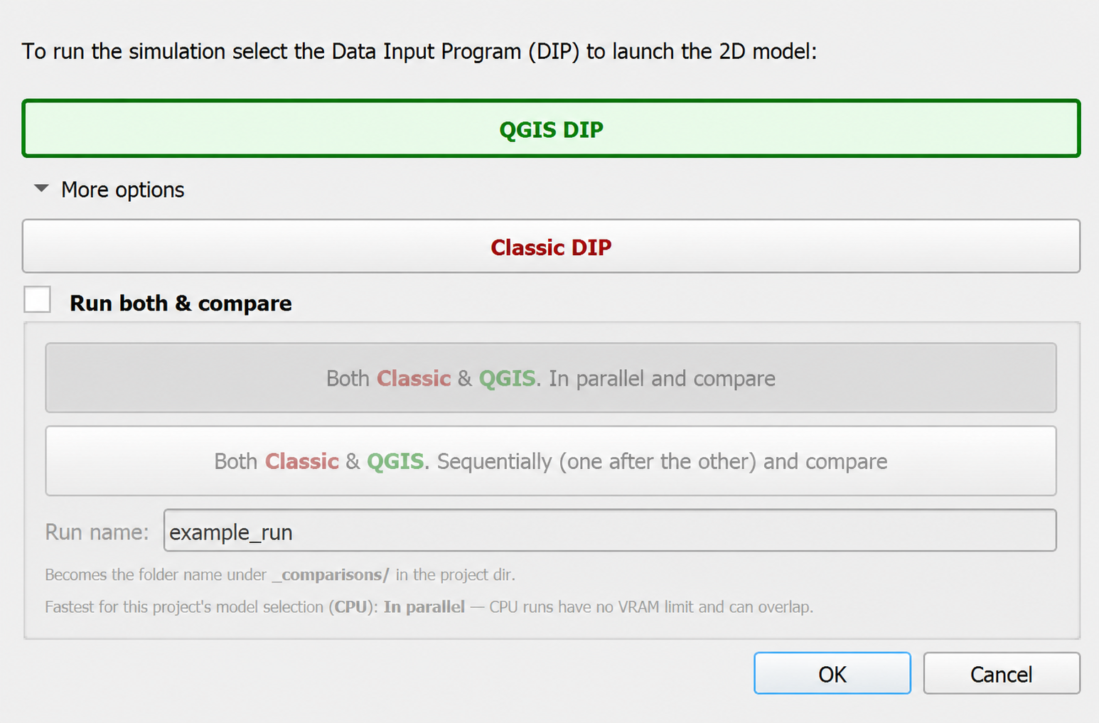

   With QGIS DIP selected, the current interface is shown below: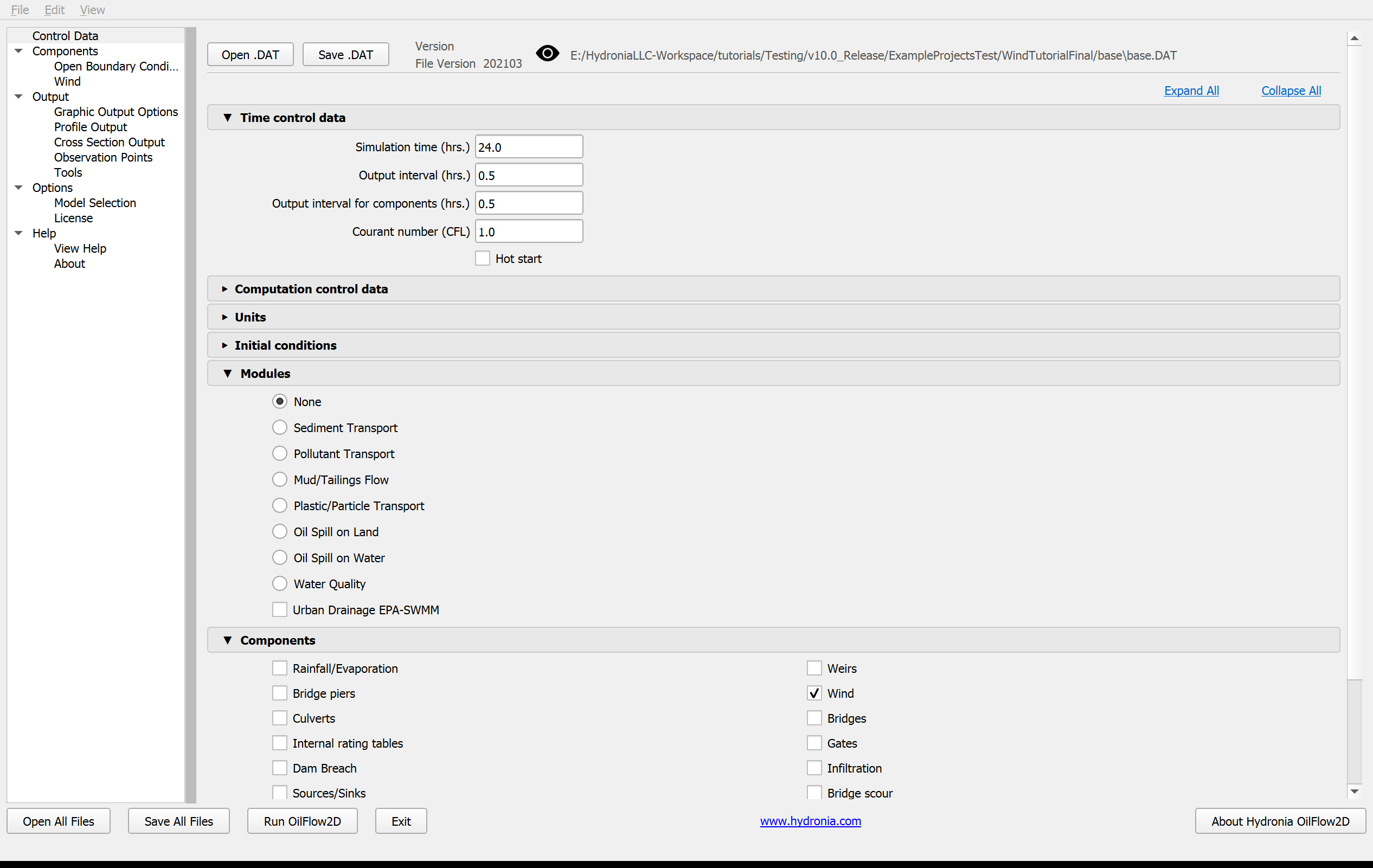

   

   QGIS DIP and Classic DIP use the same project settings, but their interfaces look different. Older standalone or non-maintenance versions may open Classic DIP automatically. The project-specific Classic DIP settings and Run steps below are retained.

Running the model

After exporting the files, Hydronia Data Input Program is loaded with the project file from the 'WindTutorial.DAT' example and shows the Control Data panel.

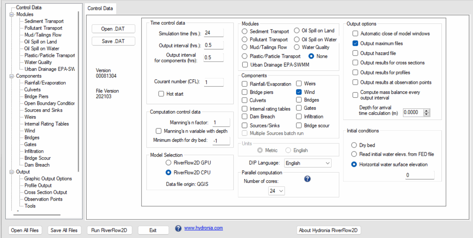
1. Enter the information as illustrated in Figure 15.7 The following Classic DIP Control Data panel is retained as a legacy values reference:

   

2. Verify that the Wind component is selected.

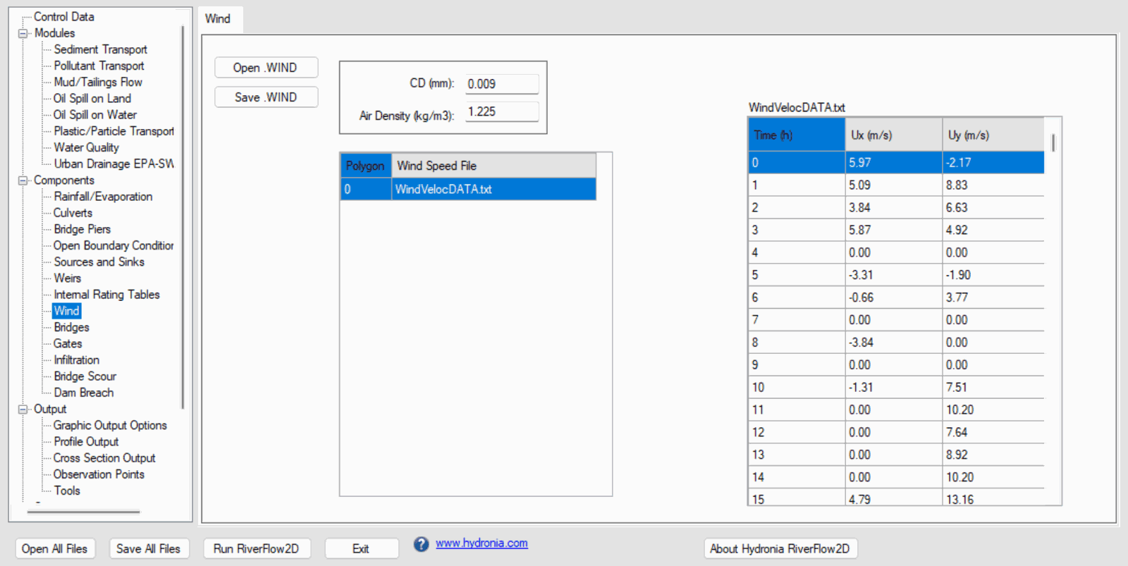
3. Select the Wind component from list in the left side of the panel. The window with the information of the wind parameters will appear as can be seen in the figure below:

   

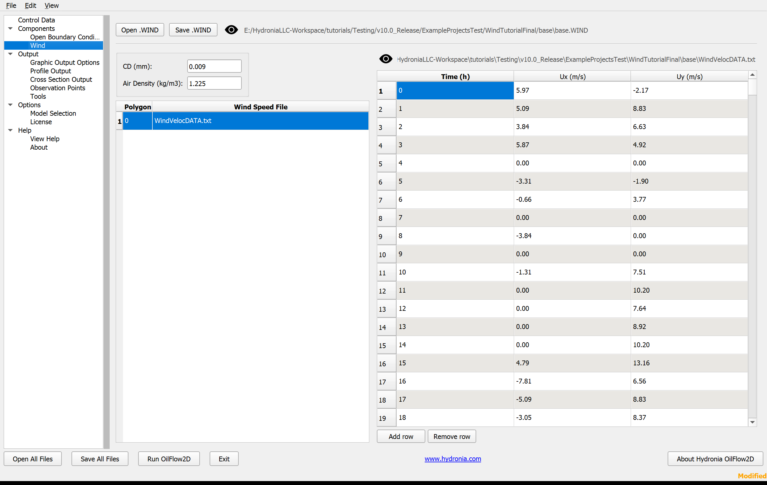
   The following Classic DIP Wind panel is retained as a legacy values reference:

   

4. Verify that the simulation time is set to 24 hours and the output interval is set to 0.5 hours.

5. Verify that the Initial conditions is set to Horizontal water surface elevation and 0 on the text box. Leave all other parameters at their default values.

6. Click on the Run OilFlow2D button in the lower section of Hydronia Data Input Program.

7. Save the changes with the same name as the 'base.DAT' file, then a window will appear indicating that the model started running.

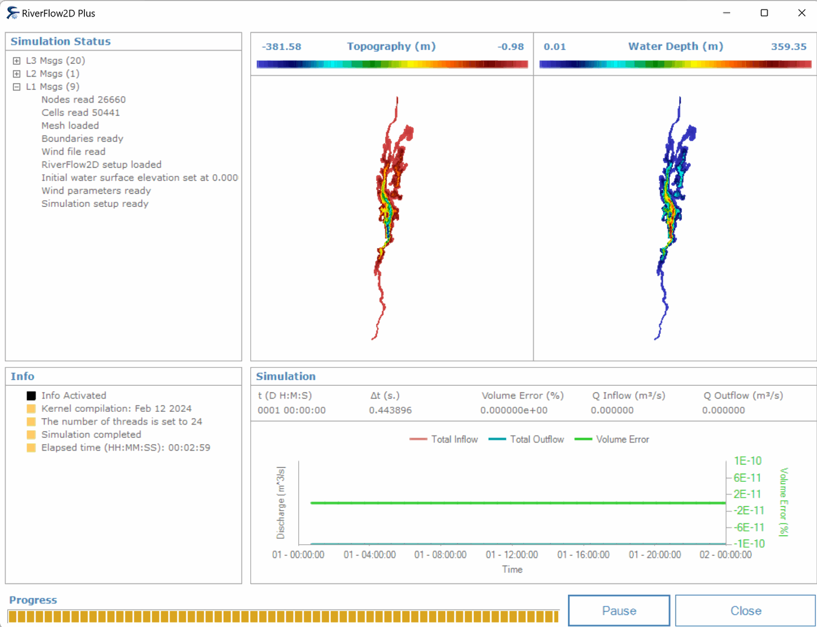
The model window that appears during the run model shows several runtime parameters.

Check the wind output files

The model creates the following files for each output time as defined in the Control panel:

'CELL_TIME_METRIC_DDDD_HH_MM_SS.TEXTOUT' (Metric Units) or

'CELL_TIME_ENG_DDDD_HH_MM_SS.TEXTOUT' (English Units)

where DDDD indicates the day, HH, hour, MM minutes and SS seconds.

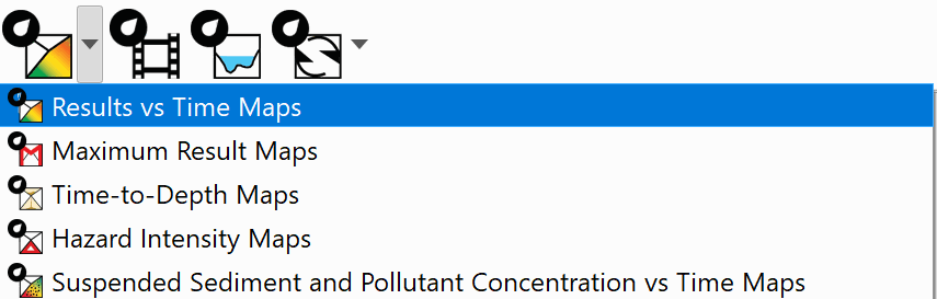
In these files, columns 1, 2 and 3 report the velocity components in Vx, Vy and the module respectively. We can visualize the water velocity fields generating layers either in raster or vectorial format from the aforementioned files using the Maps of Results vs Time tool.

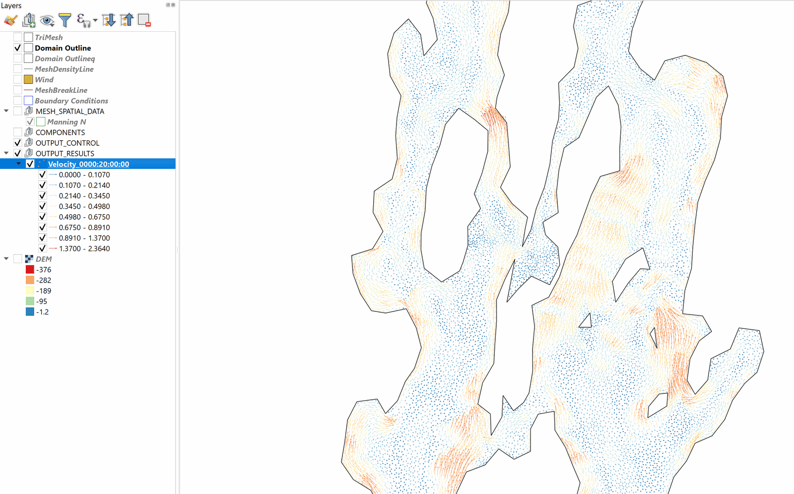
The following figure shows the water velocity field map for time 0000:20:00:00:

This concludes the Wind driven circulation tutorial.