Oil spills in Coastal Areas. Part I: Coastal Hydrodynamics

This tutorial guides in the application of OilFlow2D to simulate oil spills in a coastal area. The first part explains how to setup and run the hydrodynamic stage, where the model is used to generate the velocity field in the area. The second part, included in a separate chapter, explains how to enter the spill locations, and other oil data to simulate oil trajectories and fate.

Tutorial data

Before starting the project with QGIS. It is recommended to create a folder that will contain all the necessary data such as the boundary condition files, the elevation data files, either in ASCII or in raster format, etc.

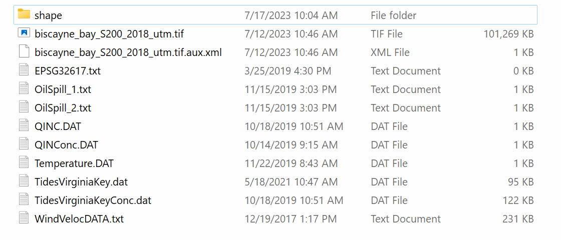
The files required to follow this tutorial can be extracted from the 'ExampleProjects' zip file under the 'OilSpillsInABayPart1' folder. This zip file is downloaded separately from your installation materials.

The folder contains the files shown:

Starting QGIS

The first step is to start the QGIS software. After loading the QGIS, you will get a window is similar to the one shown below:

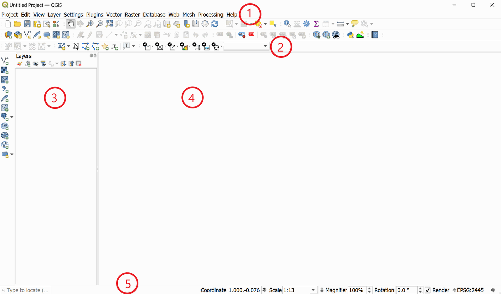
Note the tool bar contains icons that give access to all the OilFlow2D components. Some of the icons have a drop down list that allow getting to more tools.

Start a new OilFlow2D project

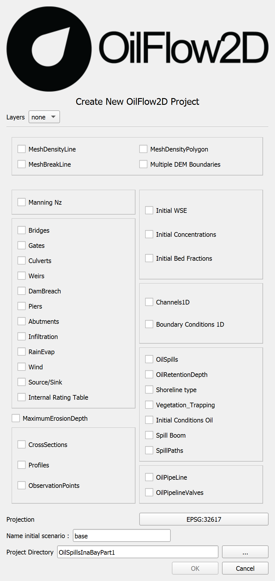
1. To create a new OilFlow2D project, click on the New OilFlow2D Project button in the toolbar. A dialog window appears where you select the optional component layers, the Coordinate Reference System (CRS), the initial scenario name, and the project directory.

2. Select None in the Layers drop down menu.

3. Select the Projection button and select: Coordinate Reference System (CRS) EPSG 32617 corresponding to WGS 84 / UTM zone 17N - Projected (meters), and click OK.

4. Keep Name initial scenario set to base. Click the "..." button and choose the OilSpillsInaBayPart1 folder for the Project Directory. This is the folder where the model will write all results and output files.

5. After clicking OK, the layer templates are created, and displayed on the Layers Panel:

   

   OilFlow2D will use the unit system as that defined in the projection you selected. If the projection has coordinates in feet, units will be set to English. If the projection coordinates are in meters, units will be set to Metric or SI.

6. On the QGIS Project menu, click Save, to save the project assigning the name OilwPart1, in the same directory that you previously selected in the Create New Project dialog above.

Load elevation data

OilFlow2D uses elevation data in raster format. For instance, to load an ASCII grid file, from the Layer menu, click Add Layer, and then click Add Raster Layer.... You may also click the Add Raster Layer button .

The following dialog will appear where you can select the raster file containing elevations. In this case, select biscayne_bay_S200_2018_utm.tif from ExampleProjects\OilSpillsInABayPart1\DATA.

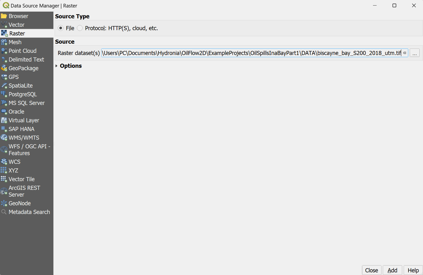
Click Add, Close the dialog and click on the Zoom Full button .

The raster will be displayed on the screen, by default it is rendered in gray gradient. Right-clicking on the label of the created layer and selecting Properties allows changing the rendering style for a more informative color palette. When changed to Singleband psudocolor it appears as shown:

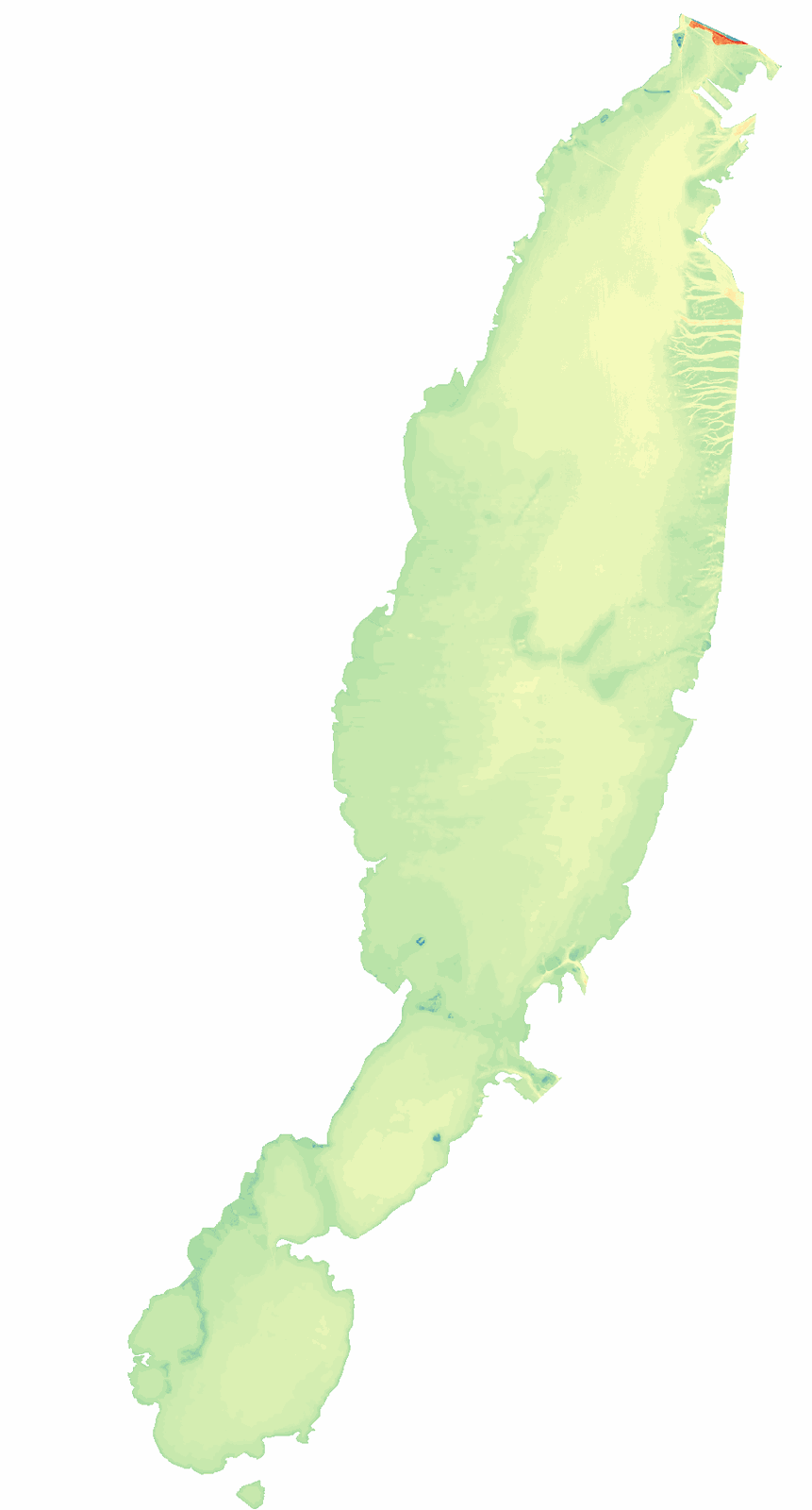
It is convenient to move the raster layer to the end of the list of layers, thus it does not interfere with the display of other layers.

Create the limits of the modeling area (Domain Outline)

The limits of the modeling area are defined using a polygon on the Domain Outline layer. To create it do as follows:

1. Click the Domain Outline layer to activate it and then click Toggle Editing (pencil) in the toolbar:

   

2. Clicking on the button activates the rest of the editing buttons. Now click the Add Polygon Feature tool which is the bean looking polygon .

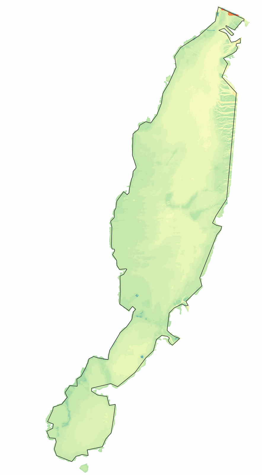
   Proceed to delineate the outline of the polygon by marking the vertices clicking with the left mouse button.

   Make sure that the polygon is contained within the limits of the raster layer since OilFlow2D will not extrapolate elevations to areas that are outside of the available data on the raster layer.

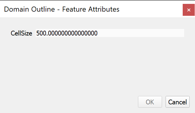
3. To finalize and close the polygon, right-click anywhere on the screen. A dialog window to input the cell size attribute of the newly created polygon. The value for the reference size of the mesh cell is indicated. Enter a value of 500 m.

   

   If you want to make any correction to the polygon, use the Node tool to move, add or remove nodes as necessary.

4. Save the polygon by clicking the Save button .

   and click on Toggle Editing icon to deactivate the layer edit mode and complete the Domain Outline.

Generating the triangular-cell mesh

Now that the Domain Outline layer has been created, proceed to create the mesh.

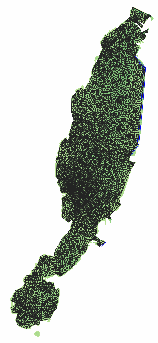
To generate the mesh, click on the icon .

The following figure shows the generated mesh. You will also find the Layers panel one new layers: Trimesh :

Setting the boundary conditions

In this tutorial we will define tidal stage condition at open boundaries. To define the tide boundary condition do as follows:

1. Click the Toggle Editing button to add the polygons that are going to indicate the nodes on which the inflow condition is imposed.

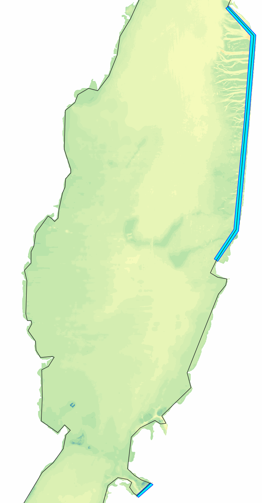
2. Draw a polygon that includes the nodes or vertices at the lower end of the mesh as indicated in the figure:

   

3. To finish the polygon, right-click on the last vertex. A window to enter the attributes of the newly created polygon is displayed. It is important that the boundary condition polygon would cover completely the inflow/outflow segment.

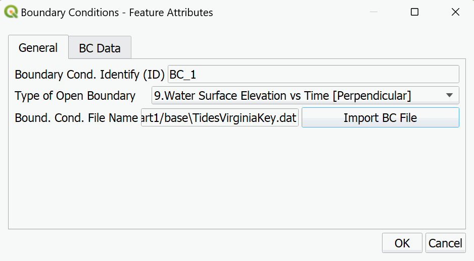
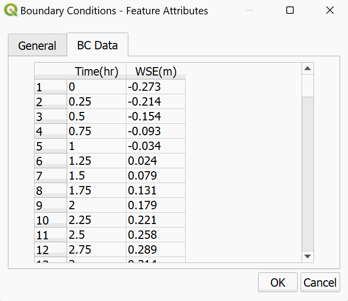
4. In the window the (Boundary Cond. ID) is BC_1, and the boundary condition Type: 9. Water Surface Elevation vs. Time[Perpendicular].

   

   

5. Repeat the process for other tidal boundaries as necessary.

There are no outflow conditions in this case, since the open boundaries will consider inflow and outflow though the tidal cycle.

Assigning Manning's n roughness coefficients

Manning's coefficients are used in OilFlow2D to represent the terrain roughness. To assign Manning's n values, we will enter polygons with particular n's. There can be as many polygons as required to reproduce the spatial variability of this parameter. In this example, a single polygon will be used for the entire area.

1. Select the Manning N layer and click the Toggle Editing button .

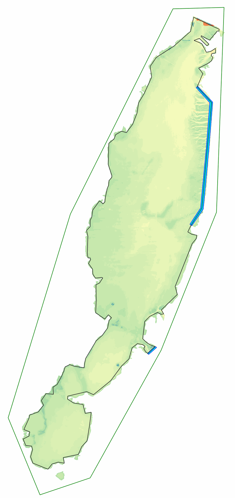
2. Draw the polygon around the entire domain taking care that it covers all the cells. You should have an image like the one shown below:

   

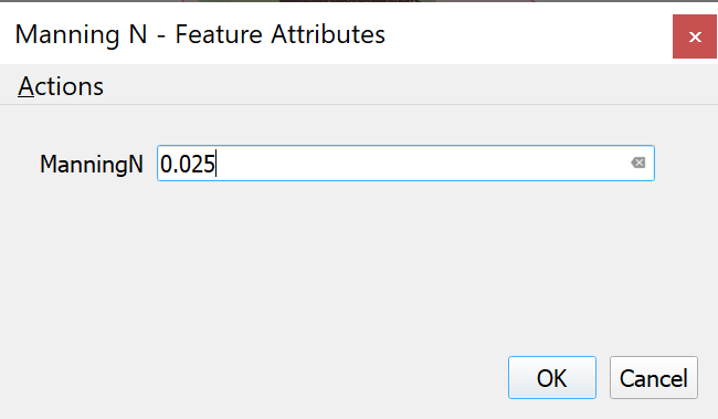
3. Close the last vertices on the polygon by right-clicking on the desired position. The following dialog window is presented where you must input the Manning's n value associated to the polygon (0.025):

   

4. Click the Save icon and then click the Editing Tool icon to deactivate editing mode.

Exporting the files to OilFlow2D and running the model

Once the layers with the input information to the model have been created, the next step is to run the tool that exports the data files in the proper format required by OilFlow2D. The process is as follows:

1. Unselect the MeshDensityLine and MeshBreakline layers, since they are not used in this example.

2. Run the Export Hydrodynamic OilFlow2D plugin:

   

3. A dialog window is presented, where we will indicate the raster layer Magdalena containing the Digital Elevation Model (DEM).

4. Click OK to start the export process.

   

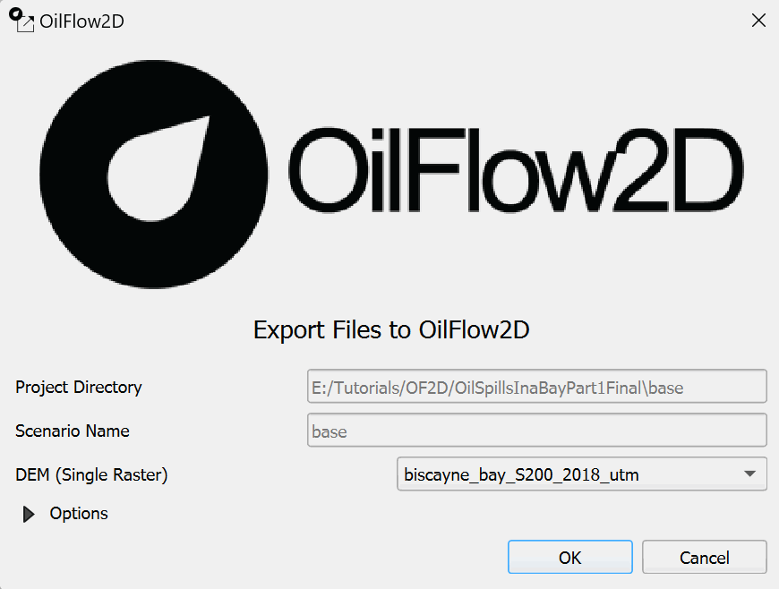
   While exporting the data, you will be able to see the task progress at the top of the message bar. After export completes, version 10 and later users see the Open DIP dialog. QGIS DIP is selected by default; click OK to open it inside QGIS. To use the historical standalone option, expand More options, select Classic DIP, and then click OK.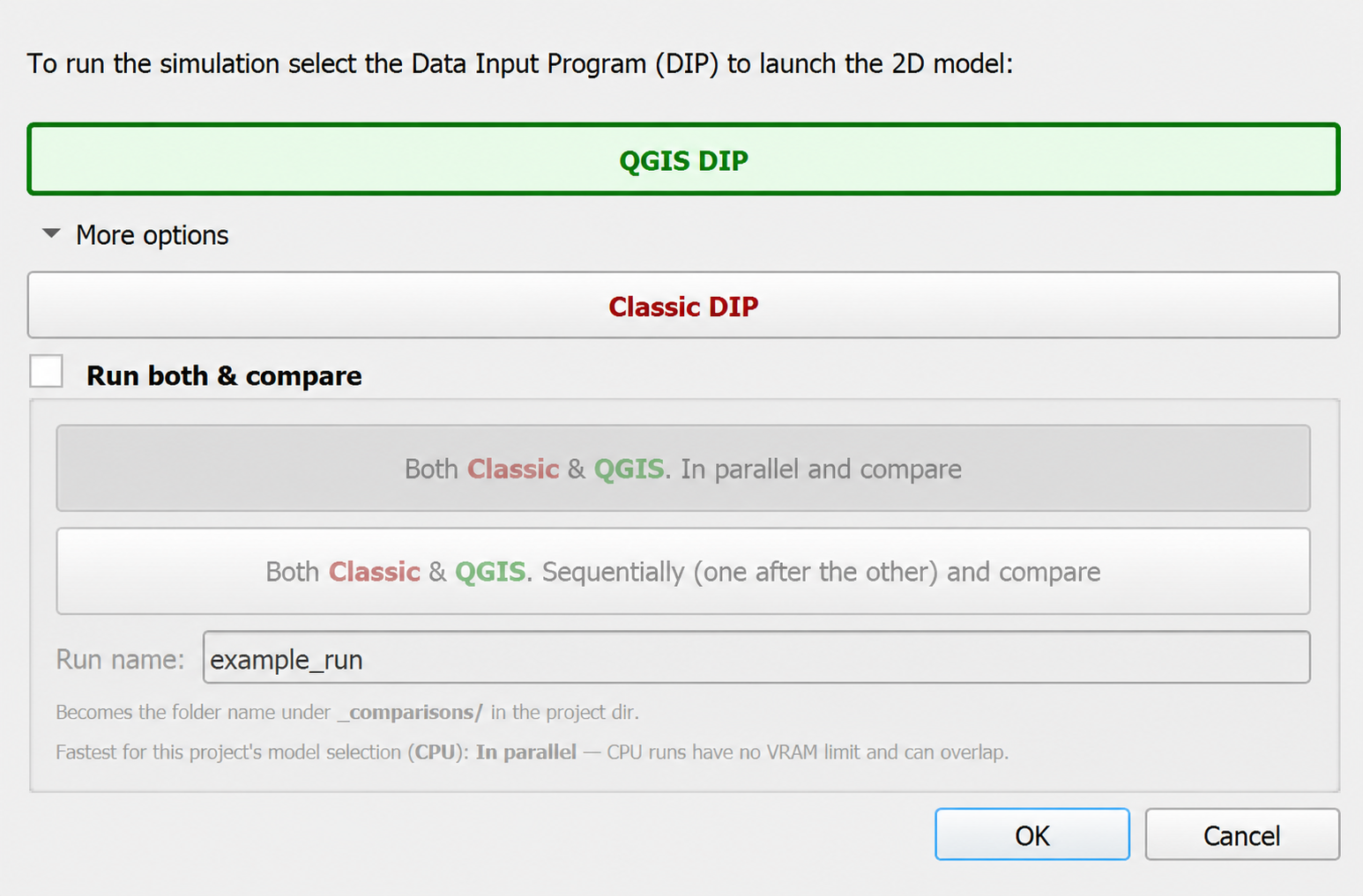

   With QGIS DIP selected, the current interface is shown below: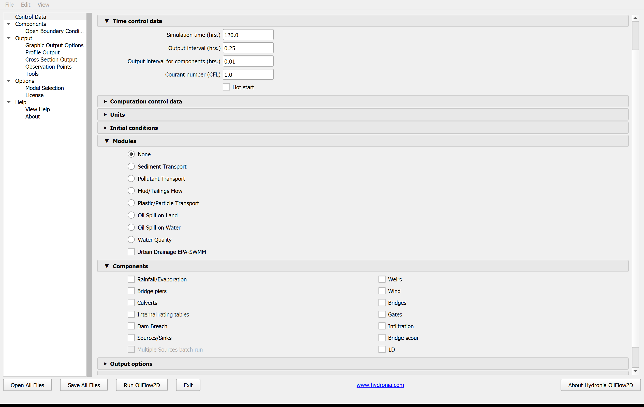

   

   QGIS DIP and Classic DIP use the same project settings, but their interfaces look different. Older standalone or non-maintenance versions may open Classic DIP automatically. The project-specific Classic DIP settings and Run steps below are retained; in this case, base.DAT should already be set.

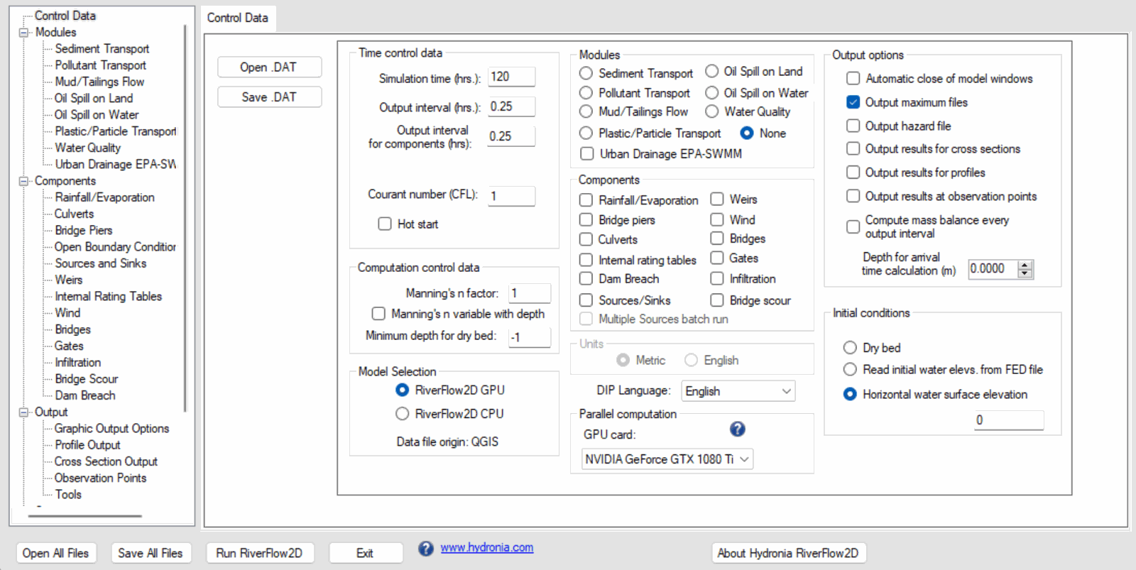
5. Enter the parameters as shown:

   The following Classic DIP configuration is retained as a legacy values reference:

   

6. Then click the Run OilFlow2D button to run the model.

7. A dialog box will appear asking to save your changes, click [Yes]. By default it will use the name of the Scenario as the name of the .dat file. Confirm to overwrite the file.

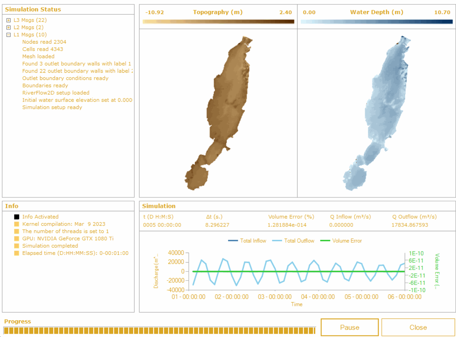
8. A few console windows will appear to initiate the model, then an image similar to the one shown below should appear.

   

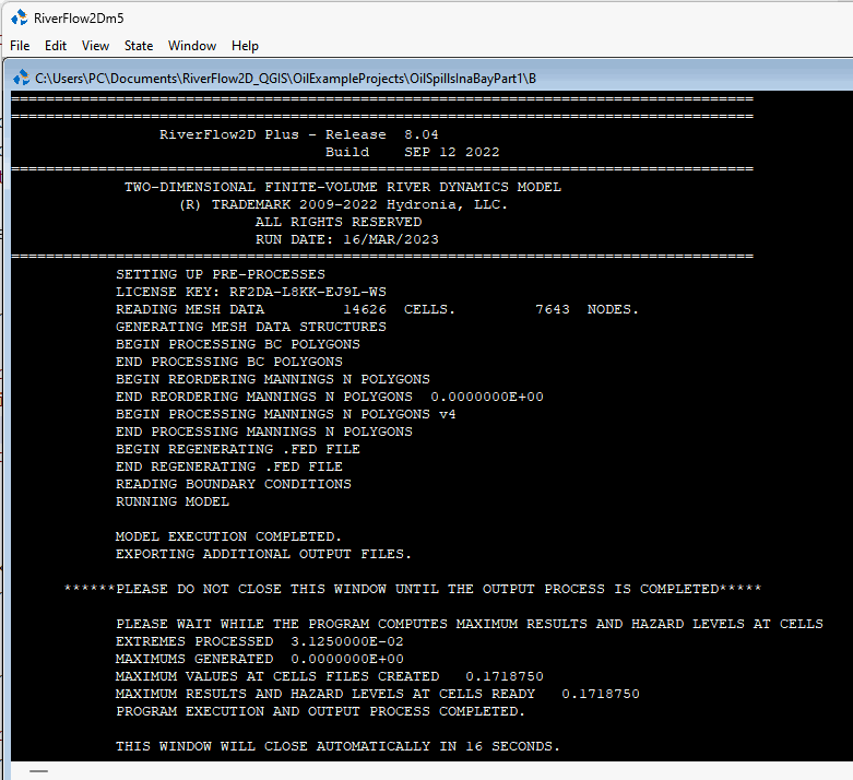
9. When you have finalized reviewing the information included in this window, close it. The following post processing window will appear indicating the final post-processed task performed by the OilFlow2D model. The window will close automatically.

   

Creating an Animation of the Velocity Field in the Bay

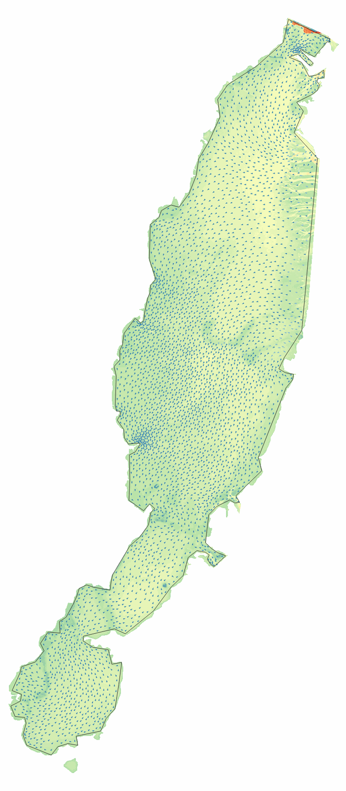
To check the model results we can create an animation of the velocity field in the bay using the following procedure:

1. Select the Animation tool :

   Wait for the animation to load. It will appear in the Animation list.

2. On the Animation panel, click Add Layer, and select the 'Velocity Field'

3. Then on the Animation panel, select the Velocity_field layer and click to view the animation

   To see the animation, the layer needs top be moved above the DEM and / or other satellite map layers.

   

This concludes the tutorial Oil spills in a coastal area. Part I: Coastal Hydrodynamics.